Welcome to my Open Notebook

This is an Open Notebook with Selected Content - Delayed. All content is licenced with CC-BY. Find out more Here.

ONS-SCD.png

notes-on-spatial-stats-meeting-with-sarunya-sujaritpong

  • Yesterday I met with Sarunya Sujaritpong a PhD student working with spatially structured time-series models as described previously
  • Her supervisor Keith Dear has given me a lot of good stats advice in the past and one bit I keep thinking about is that a time series model can be fit for multiple spatial areal units of the same city and residual spatial auto-correlation in the errors should not be too much of a concern
  • The problem would be if you get strong spatial autocorrelation of the residuals this indicates that the assumption of independent errors is violated and you will have tighter confidence intervals around the coefficients of interest than is really the case, inflating the signficance estimated for the relative risk
  • The beta coefficient itself shouldn’t be affected.
  • So long as biostatisticians like Keith are comfortable with not addressing this issue in spatially structured time-series that is great but I see people are starting to include this in their models
  • To date I’ve mostly seen it done in spatial (cross sectional) data analysis, not spatial times-series
  • I’m preparing for the day when I might need to address this for a reviewer and would like to know what to do about it in case that happens
  • So I asked Sarunya for a discussion about her research

Sarunya’s model is essentially like this

R Code:

fit <- glm(deaths ~ pollutant1 + pollutant2 + pollutant ... +
       ns(temp, df) + ns(humidity, df) +
       ns(time, df = 7*numYears) +
       SLA * ns(time, df = 2),
       data = analyte, family = poisson
       )

  • SLA is Statistical Local Area (now called SA2, like a suburb)
  • Sarunya explained that the research question was if the magnitude of the coeff on pollutant1 differed between this model and the old style of model where an entire city is used as the unit of analysis per day and exposure estimates are calculated as averages across several monitoring stations in the city
  • turns out that this comparison is still valid EVEN IF THE STANDARD ERROR IS BIASED DUE TO RESIDUAL SPATIAL AUTOCORRELATION
  • therefore this study avoids the issue by it’s intentional design to compare betas not se
  • Interestingly Sarunya explained that the stats theory suggests that even if the exposure precision is increased (exposure misclassification bias is decreased) the se on the beta will not be affected.
  • this is fascinating in itself, but a separate issue for another post

Conclusions

  • So it looks like the extent a study might need to consider the issue of potential residual spatial autocorrelation depends alot on what questions are being asked and what inferences will be attempted from the results
  • if the aim of the study is to estimate the magnitude AND CONFIDENCE INTERVALS of an exposure’s relative risk (especially some novel exposure such as interstellar space dust across the suburbs) then the issue might become important to address.

THANKS Sarunya!

Posted in  spatial dependence


if-disease-incidence-varies-with-age-control-for-it

  • today I was in a meeting where the discussion turned to maps of crude incidence rates, age-standardised rates and regression models controlling for age
  • If disease incidence does not vary with age then there is not much point in controlling for this,
  • apart from the work done in exploratory data analysis to ascertain whether or not this is the case
  • I proposed that if you’ve done all the work on age-specific rates needed to test if incidence varies with age, then you might as well present age adjusted rates seeing as you’ve already done the work anyway

An example

  • The project is highly confidential due to the nature of the data
  • We;ll call the study location South Kingsland to protect the identity

R Code:

# get spatial data
require(swishdbtools) # github package, under
                      # swish-climate-impact-assessment

Tab1 <- read.csv("data/dataset.csv", sep= ",", header = TRUE, stringsAsFactor = F)
Tab1 <- as.data.frame(table(Tab1$SLA))
nrow(Tab1)
write.csv(Tab1, "data/SLA.csv", row.names = F)
load2postgres("data/SLA.csv", schema="ivan_hanigan", tablename="sla", ip = "brawn.anu.edu.au",
              db = "gislibrary", pguser = "ivan_hanigan", printcopy = F)


ch  <- connect2postgres2("gislibrary")
sql_subset(ch, "ivan_hanigan.sla", eval = T, limit = 10)


sql_subset(ch, "abs_sla.qldsla01", select =  "sla_name, st_y(st_centroid(geom))", eval = T, limit = 10)
dbSendQuery(ch,
  "select sla_name, geom
  into southkingsland
  from abs_sla.qldsla01 t1
  join
  sla t2
  on t1.sla_name = t2.var1;
  alter table southkingsland add column gid serial primary key;
  ")
# these are missing from spatial data
## 42                      West End                          <NA>
## 43                OVERSEAS-OTHER                          <NA>
## 44                  Yarrabah (S)                          <NA>
## 45     Rowes Bay-Belgian gardens                          <NA>

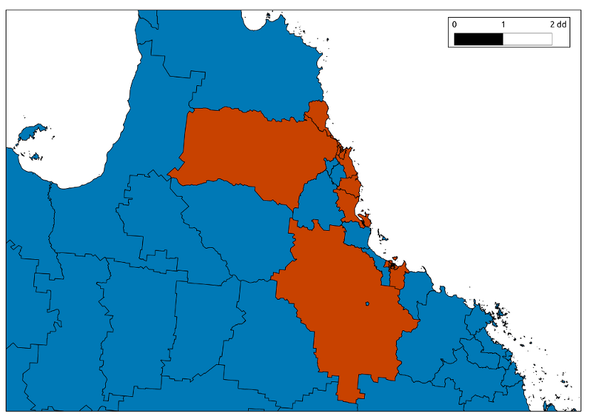
visualise with QGIS

southkingsland.png

R Code:

# func
require(plyr)
 
# load
Tab2 <- read.csv("data/dataset.csv", sep= ",", header = TRUE, stringsAsFactor = F)
names(Tab2)
# [1] "SLA"       "agegrp"    "Sex"       "district"  "dm"        "ninf"     
# [7] "popSLA"    "Month"     "Year"      "groupyear"
test_sla  <- names(table(Tab2$SLA)[1])
subset(Tab2, SLA == test_sla & Year == 2001 & agegrp == 1 & Sex == "MALE")
subset(Tab2, SLA == test_sla & Year == 2001 & agegrp == 1 & Sex == "FEMALE")

# clean
summary(Tab2)
## remove any SLA with NA populations
Tab2 <- Tab2[which(!is.na(Tab2$popSLA)),]     
 
# do
## first total cases by annualised pop
analyte  <- ddply(Tab2, c("SLA", "Year", "agegrp", "Sex"), summarise,
                  ninf=sum(ninf),
                  popSLA=mean(popSLA)
                  )
#str(analyte)

#subset(analyte, SLA == test_sla)
subset(analyte, SLA == test_sla & Year == 2001 & agegrp == 1)
 
## now annual totals for study region
analyte2  <- ddply(analyte, c("Year", "agegrp"), summarise,
                  ninf=sum(ninf),
                  popSLA=sum(popSLA)
                  )
str(analyte2)

qc <- subset(analyte2,  Year == 2001)
qc
sum(qc$popSLA)
 
## now totals
qc  <- ddply(analyte2, c("Year"), summarise,
             ninf=sum(ninf),
             popSLA=sum(popSLA)
             )
qc
sum(qc$ninf)
mean(qc$popSLA)

## totals by age
subset(analyte2,  agegrp == 1)
analyte3  <- ddply(analyte2, c("agegrp"), summarise,
                  ninf=sum(ninf),
                  popSLA=mean(popSLA)
                  )
analyte3
sum(analyte3$popSLA)
analyte3$asr  <- (analyte3$ninf / analyte3$popSLA) * 1000
analyte3

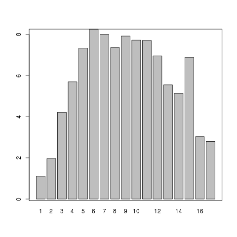
png("graphs/south-kingsland-age-specific-rates.png") 
mp <- barplot(analyte3$asr, names.arg = analyte3$agegrp)
box()
dev.off()

Plot Age Specific Rates

Great so with that bit of work we should have an idea of the variation of incidence by age

south-kingsland-age-specific-rates.png

Results and Discussion

  • It looks like the incidence does vary with age
  • TODO make graphs per year (the scale of the above graph is wrong - decades in the numerator but annualised pops in the denominator)
  • TODO make graphs by city, by sex
  • age-standardised rates probably need different age categories, only 4 or 5?
  • worth commenting on the liklihood that age is not important for time-series models at the city scale, unless age structure changes substantially over time (this is an analysis for the spatial pattern only)

Clean up database!

dbSendQuery(ch, "drop table sla")
dbSendQuery(ch, "drop table southkingsland")

Posted in  research methods


morpho-and-reml-boilerplate-streamline-the-process-of-metadata-entry

Disentangle Things

1 morpho-and-reml-boilerplate-streamline-the-process-of-metadata-entry

1.1 Background

  • The Morpho/Metacat system is great for a data repository
  • Morpho also claims to be suitable for Ecologists to document their data
  • But in my experience it leaves a little to be desired in ease of use for both purposes
  • Specifically the speed that documentation can be entered into Morpho is slow
  • This post is a first attempt to create some boilerplate code to quickly generate EML metadata using REML.

1.2 Speed and Rigour

As I noted in a previous post, there are [two types of data documentation workflow](http://ivanhanigan.github.io/2013/10/two-main-types-of-data-documentation-workflow/).

  • GUI
  • Programatic

I also think there are two types of users with different motivations and constraints:

  • 1) Data Analysts
  • 2) Data Librarians

1.3 Analysts can often trade-off completeness of documentation for speed

In my view the Analysts group of users need a tool that will very rapidly document their data and workflow steps and can live with a bit less rigour in the quality of documentation. Obviously this is not ideal but seems an inevitable trade-off needed to enable analysts to keep up the momentum of the data processing and modelling without getting distracted by tedious (and potentially unnecessary) data documentation tasks.

1.4 Librarians produce gold plated documentation and can take longer to produce this

On the other hand the role of the Librarian group is to produce documentation to the best level possible (given time and resource constraints) the datasets and methodologies that lead to the creation of the datasets. For that group Rigour will take precedence and there will be a trade-off in terms of the amount of time needed to produce the documentation.

1.5 An example

As an example of the two different groups, an analyst working with weather data in Australia may want to specify that their variable "temperature" is the average of the daily maxima and minima, but might not need to specify that the observations were taken inside a Stevenson Screen, or even if they are in Celsius, Farenhiet or Kelvin. They will be very keen to start the analysis to identify any associations between weather variables and the response variable they are investigating. The data librarian on the other hand will be more likely to need to include this information so that the users of the temperature data do not mis-interpret it.

1.6 Embracing Inaccuracy and Incompleteness

  • I've been talking about this for a while got referred to this document by Ben Davies at the ANUSF

[http://thedailywtf.com/Articles/Documentation-Done-Right.aspx](http://thedailywtf.com/Articles/Documentation-Done-Right.aspx)

  • It has this bit:
  
   
Embracing Inaccuracy and Incompleteness 
    
The immediate answer to what’s the right way to do documentation is
clear: produce the least amount of documentation needed to facilitate
the most understanding, and be very explicit about which documentation
is to be maintained and which is to be archived (i.e., read-only and
left to rot).
  • Roughly speaking, a full EML document produced by Morpho is a bit like a whole bunch of cruft that isnt needed and gets in the way (and is more confusing)
  • Whereas a minimal version Im thinking of covers almost all the generic entries providing the "minimum amount of stuff to make it work right".

1.7 Aim

  • This experiment aims to speed up the creation of a minimal "skeleton" of metadata to a level that both the groups above can be comfortable with AS A FIRST STEP.
  • It is assumed that additional steps will then need to be taken to complete the documentation, but the automation of the first part of the process should shave off enough time to suit the purposes of both groups
  • It is an imperative that the quick-start creation of the metadata does not end up costing the documentor more time later on down the track if they need to go back to many of the elements for additional editing.

1.8 Step 1: load a simple example dataset

I've been using a [fictitious dataset from a Statistics Methodology paper by Ritschard 2006](http://ivanhanigan.github.io/2013/10/test-data-for-classification-trees/). It will do as a first cut but when it comes to actually test this out it would be good to have something that would take a bit longer (so that the frustrations of using Morpho become very apparent).

  #### R Code:
      # func
      require(devtools)
      install_github("disentangle", "ivanhanigan")
      require(disentangle)
      # load
      fpath <- system.file(
          file.path("extdata", "civst_gend_sector_full.csv"),
          package = "disentangle"
          )
      data_set <- read.csv(fpath)
      summary(data_set)
      # store it in the current project workspace
      write.csv(data_set, "data/civst_gend_sector_full.csv", row.names = F)


## | divorced/widowed: 33 | female:132 | primary  :116 | Min.   : 128.9 |
## | married         :120 | male  :141 | secondary: 99 | 1st Qu.: 768.3 |
## | single          :120 | nil        | tertiary : 58 | Median : 922.8 |
## | nil                  | nil        | nil           | Mean   : 908.4 |
## | nil                  | nil        | nil           | 3rd Qu.:1079.1 |
## | nil                  | nil        | nil           | Max.   :1479.4 |

1.9 Step 2 create a function to deliver the minimal metadata object

  • the package REML will create a EML metadata document quite easily
  • I will assume that a lot of the data elements are self explanatory and take column names and factor levels as the descriptions

1.10 remlboilerplate-code

################################################################
# name:reml_boilerplate
 
# func
if(!require(reml)) {
  require(devtools)
  install_github("reml", "ropensci")
  } 
require(reml)

reml_boilerplate <- function(data_set, created_by = "Ivan Hanigan <ivanhanigan@gmail.com>", data_dir = getwd(), titl = NA, desc = "")
{

  # essential
  if(is.na(titl)) stop(print("must specify title"))
  # we can get the col names easily
  col_defs <- names(data_set)
  # next create a list from the data
  unit_defs <- list()
  for(i in 1:ncol(data_set))
    {
      # i = 4
      if(is.numeric(data_set[,i])){
        unit_defs[[i]] <- "numeric"
      } else {
        unit_defs[[i]] <- names(table(data_set[,i]))          
      }
    }
  # unit_defs
  
  ds <- data.set(data_set,
                 col.defs = col_defs,
                 unit.defs = unit_defs
                 )
  #str(ds)

  metadata  <- metadata(ds)
  # needs names
  for(i in 1:ncol(data_set))
    {
      # i = 4
      if(is.numeric(data_set[,i])){
        names(metadata[[i]][[3]]) <- "number"
      } else {
        names(metadata[[i]][[3]]) <- metadata[[i]][[3]]
      }
    }
  # metadata
  oldwd <- getwd()
  setwd(data_dir)
  eml_write(data_set, metadata,
            title = titl,  
            description = desc,
            creator = created_by
            )
  setwd(oldwd)
  sprintf("your metadata has been created in the '%s' directory", data_dir)
  }

1.11 remlboilerplate-test-code

################################################################
# name:reml_boilerplate-test

analyte <- read.csv("data/civst_gend_sector_full.csv")
reml_boilerplate(
  data_set = analyte,
  created_by = "Ivan Hanigan <ivanhanigan@gmail.com>",
  data_dir = "data",
  titl = "civst_gend_sector_full",
  desc = "An example, fictional dataset"
  )

dir("data")

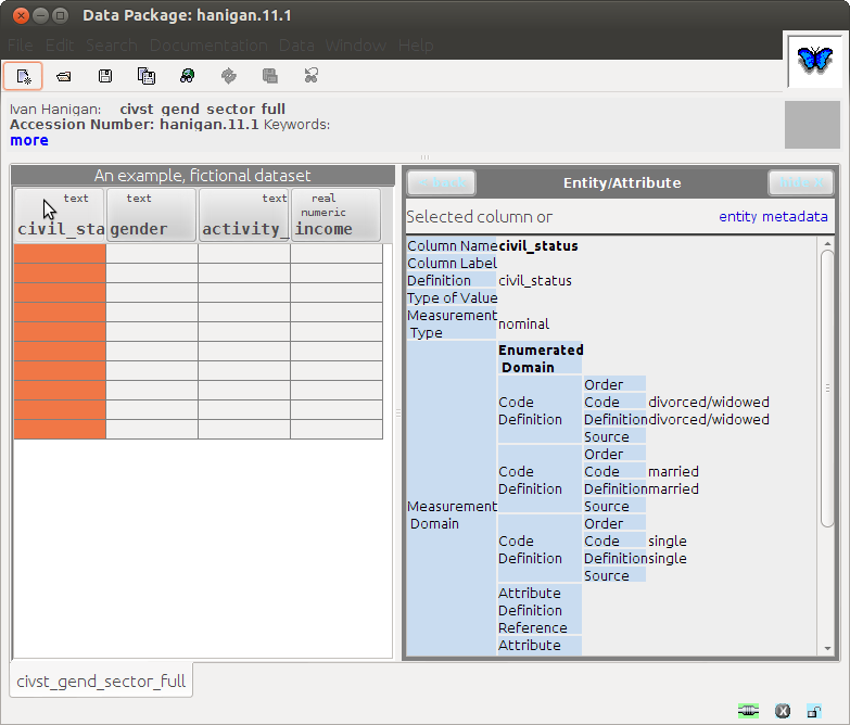
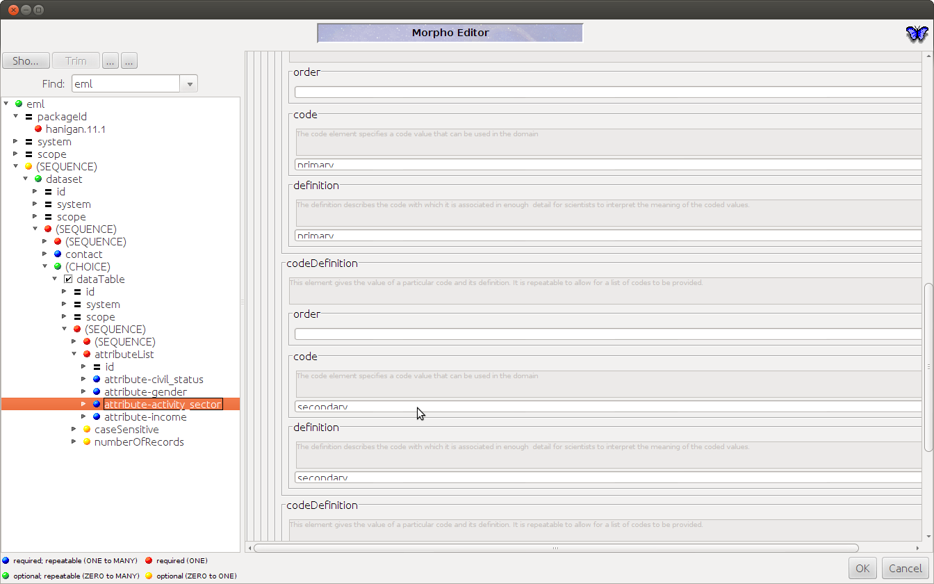
1.12 Results: This loads into Morpho with some errors

  • Notably unable to import the data file

morpho-reml-boilerplate.png

  • Also "the saved document is not valid for some reason"

morpho-reml-boilerplate2.png

1.13 Conclusions

  • This needs testing
  • A real deal breaker is if the EML is not valid
  • In some cases not having the data table included will be a deal breaker (ie KNB repositories designed for downloading complete data packs
  • A definite failure would be that even if it is quicker to get started if it takes a long time and is difficult to fix up it might increase the risk of misunderstandings.

</html>

Posted in  Data Documentation


counting-number-of-consecutive-months-in-drought

I got this question today from a Drought researcher:

Question:

There a table with 62 years * 12 months of rain data in mm. We
calculated the cumulative distribution using ecdf: empirical
cumulative distribution function. So the table looks like this:
Year Jan Feb Mach (…) each cell contains the cum dist.
  
We also got the number of months per year with less than X mm of
rain. But he needs to know how many months are between the
drought months, regardless the year. So, I thought that
converting the data into a ts was going to facilitate the task,
but it doesn’t, because now I don’t’ have columns and rows any
longer.
 
How do I handle a ts object to do for example an ifelse?

I answered:

This looks a lot like the Hutchinson Drought Index which I’ve coded up here

This is the key bit for counting consecutive months below a threshold

R Code:

x<-data$index<=-1
xx <- (cumsum(!x) + 1) * x
x2<-(seq_along(x) - match(xx, xx) + 1) * x
data$count<-x2

I got it from https://stat.ethz.ch/pipermail/r-help/2007-June/134594.html and looked in wonder at the structure and am amazed it works.

I also really like the cumulative summing version a lot

R Code:

data$sums<-as.numeric(0)
y <- ifelse(data$index >= -1, 0, data$index)
f <- data$index < -1
f <- (cumsum(!f) + 1) * f
z <- unsplit(lapply(split(y,f),cumsum),f)
data$sums <- z

Several things I’d like to change.

  • I like the idea of using a wide dataset and ecdf rather than my loop thru months
  • I’d like to look into Joe Wheatley;s approach http://joewheatley.net/20th-century-droughts/
  • I was defeated by Mike’s request to make a different threshold for breaking a drought than starting a drought. went back to a for loop

Posted in  climatic and agricultural drought


spatial-lag-and-timeseries-model-with-nmmaps

UPDATE

OLD POST

  • Today I chatted with Phil Kokic at CSIRO Mathematics, Informatics and Statistics about the way the spatially lagged neighbours variable absorbs any residual spatial correlation in the errors
  • We agreed that this is a pretty minimal attempt, not as good as a spatial error model but pretty easy to implement
  • I’ve hacked together some very very ugly code to construct the lagged variable
  • http://ivanhanigan.github.io/spatiotemporal-regression-models/#sec-3
  • There may be errors, it’s been a long day, but I won’t have a chance to check back on this till next week so I thought I’d put it out there as is.

Posted in  spatial dependence