A fictitious sample dataset
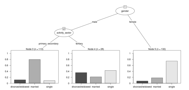
For discussion, I’ll use a fictional example dataset that I’m using to work through some statistical theory related to Classification and Regression Trees (CART). In the motivating example use case we are interested in predicting the civil status (married, single, divorced/widowed) of individuals from their sex (male, female) and sector of activity (primary, secondary, tertiary). The data set is composed of 273 cases.
The data (and related statistical theory) come from:
-
Ritschard, G. (2006). Computing and using the deviance with classification trees. In Compstat 2006 - Proceedings in Computational Statistics 17th Symposium Held in Rome, Italy, 2006. Retrieved from This Link
-
Ritschard, G., Pisetta, V., & Zighed, D. (2008). Inducing and evaluating classification trees with statistical implicative criteria. Statistical Implicative Analysis. Studies in Computational Intelligence Volume 127, pp 397-419. Retrieved from This Link
Code:
# copy and paste the data from the PDF (Table 1 in both papers)
civst_gend_sector  <- read.csv(textConnection(
    "civil_status gender activity_sector number_of_cases
         married   male         primary              50
         married   male       secondary              40
         married   male        tertiary               6
         married female         primary               0
         married female       secondary              14
         married female        tertiary              10
          single   male         primary               5
          single   male       secondary               5
          single   male        tertiary              12
          single female         primary              50
          single female       secondary              30
          single female        tertiary              18
divorced/widowed   male         primary               5
divorced/widowed   male       secondary               8
divorced/widowed   male        tertiary              10
divorced/widowed female         primary               6
divorced/widowed female       secondary               2
divorced/widowed female        tertiary               2
"),sep = "")

# save this to my personal R utilities package "disentangle"
# for use later when I am exploring functions
dir.create("inst/extdata", recursive=T)
write.csv(civst_gend_sector, "inst/extdata/civst_gend_sector.csv", row.names = F)
That is fine and good, we can use the case weights option to include number of cases but sometimes we want to use one row per person. In the next chunk of code I;ll reformat the data, and also add another fictitious variable called income and contrive an example where a certain group earns less based on their activity sector.
Code:
df <- as.data.frame(matrix(NA, nrow = 0, ncol = 3))
for(i in 1:nrow(civst_gend_sector))
    {
    #    i <- 1
        n <- civst_gend_sector$number_of_cases[i]
        if(n == 0) next
        for(j in 1:n)
            {
              df <- rbind(df, civst_gend_sector[i,1:3])
            }

    }

df$income  <- rnorm(nrow(df), 1000,200)
# Let us say secondary men earn less
df$income[df$gender == "male" & df$activity == "secondary"]  <- df$income[df$gender == "male" & df$activity == "secondary"] - 500
str(df)
# save this for use later
write.csv(df, "inst/extdata/civst_gend_sector_full.csv", row.names = F)
Motivating reason for using these data
Classification and Regression Tree models (also referred to as Decision Trees) are one of the building blocks of data mining and a great tool for Exploratory Data Analysis.
I’ve mostly used Regression Trees in the past but recently got some work with social science data where Classification Trees were needed. I wanted to assess the deviance as well as the misclassification error rate for measuring the descriptive power of the tree. While this is a easy with Regression Trees it became obvious that it was not so easy with Classification Trees. This is because Classification Trees are most often evaluated by means of the error rate. The problem with the error rate is that it is not that helpful for assessing the descriptive capacity of the tree.
For example if we look at the reduction in deviance between the Null model and the fitted tree we can say that the tree explains about XYZ% of the variation. We can also test if this is a statistically significant reduction based on a chi-squared test.
Consider this example from page 310 of Hastie, T., Tibshirani, R., & Friedman, J. (2001). The elements of statistical learning. 2nd Edition:
- in a two-class problem with 400 observations in each class (denote this by (400, 400))
- suppose one split created nodes (300, 100) and (100, 300),
- the other created nodes (200, 400) and (200, 0).
- Both splits produce a misclassification rate of 0.25, but the second split produces a pure node and is probably preferable.
During the course of my research to try to identify the best available method to implement in my analysis I found a useful series of papers by Ritschard, with a worked example using SPSS. I hope to translate that to R in the future, but the first thing I did was grab the example data used in several of those papers out of the PDF. So seeing as this was a public dataset (I use a lot of restricted data) and because I want to be able to use it to demonstrate the use of any R functions I find or write… I thought would publish it properly.
The Tree Model
So just before we leave Ritschard and the CART method, let’s just fit the model. Let’s also install my R utilities package “disentangle”, to test that we can access the data from it.
In this analysis the civil status is the outcome (or response or decision or dependent) variable, while sex and activity sector are the predictors (or condition or independent variables).
Code:
# func
require(rpart)
require(partykit)
require(devtools)
install_github("disentangle", "ivanhanigan")

# load
fpath <- system.file(file.path("extdata", "civst_gend_sector.csv"),
                     package = "disentangle"
                     )
civst_gend_sector <- read.csv(fpath)

# clean
str(civst_gend_sector)

# do
fit <- rpart(civil_status ~ gender + activity_sector,
             data = civst_gend_sector, weights = number_of_cases,
             control=rpart.control(minsplit=1))
# NB need minsplit to be adjusted for weights.
summary(fit)

# report
dir.create("images")
png("images/fit1.png", 1000, 480)
plot(as.party(fit))
dev.off()
The Result