Welcome to my Open Notebook

This is an Open Notebook with Selected Content - Delayed. All content is licenced with CC-BY. Find out more Here.

ONS-SCD.png

tumbarumba-supersite-dem

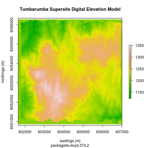
  • The first dataset I downloaded from ASN for playing around with was the Tumba Lidar.
  • I had thought it might be better to offer this as a OGC service rather than downloadable geotiff
  • just in terms of the size firstly (104MB)
  • but I also soon realised it would need some specialised tweaking which non-GIS users might struggle a bit and could avoid if the serverside data is set up by a GIS specialist (although can we assume only GIS specialists will download this kind of data)?
  • kudos to http://stackoverflow.com/questions/11966503/how-to-replace-nas-in-a-raster-object

Code:tumbarumba-supersite-dem

setwd("~/data/supersite/tumba-lidar")
require(raster)
fname  <- dir(pattern = "tif$")
fname
r  <- raster(fname)
str(r)
dfr <- as.data.frame(r)
summary(dfr)
# the -1 code looks like it might be missing?  They are around the edge.
rna <- reclassify(r, cbind(-1, 1197))
png("tumba-lidar.png")
plot(rna, col=terrain.colors(100), xlab = "eastings (m)", ylab = "northings (m)")
title("Tumbarumba Supersite Digital Elevation Model")
title(sub = "packageId=lloyd.374.2")
dev.off()
tumba-lidar.png

Alternately use a geoserver

;

  • PS the map might take a minute to show up, not sure why, might ask the sysadmin to look at the server performance

Posted in  research methods


extend-Rs-data-frame-class-with-metadata

“reml now extends R’s data.frame class by introducing the data.set class which includes additional metadata required by EML” https://github.com/ropensci/reml

and “I’d like to define a class that acts just like a data.frame, just like the data.table class does, but contains some additional metadata (e.g. the units associated with the columns) and has some additional methods associated with it (e.g. that might do something with those units) while also working with any function that simply knows how to handle data.frame objects. How might this be done?” http://carlboettiger.info/2013/09/11/extending-data-frame-class.html

Also this guys attempt was interesting (I like TraMineR too!) http://ivanhanigan.github.io/2013/11/handling-survey-data-with-r/

Posted in  research methods


a-few-best-practices-for-statistical-programming

  • John Myles White invented the ProjectTemplate R Package
  • This is a great application that helps streamline the process of creating a data analysis project
  • Recently John posted about some tips for best practices for statistical programming

Best Practices for Statistical Programming

  • Write Out a Directed Acyclic Graph (DAG)
  • Vectorize Your Operations
  • Profile your code and understand where it spends its time
  • Generate Data and Fit Models
  • Correctness: always ensure that code infers parameters of models given simulated data with known parameters.

Additional suggestions

  • Unit Testing (use testthat)
  • Create modular code with discrete chunks
  • Write functions as much as possible, put these into a personal ‘misc’ package

Posted in  research methods


add-2d-plots-of-trend-and-wiggle-to-catastrophic-regime-shifts-plot

Catastrophic Regime Shifts Visualisation

Catastrophic Regime Shifts Visualisation


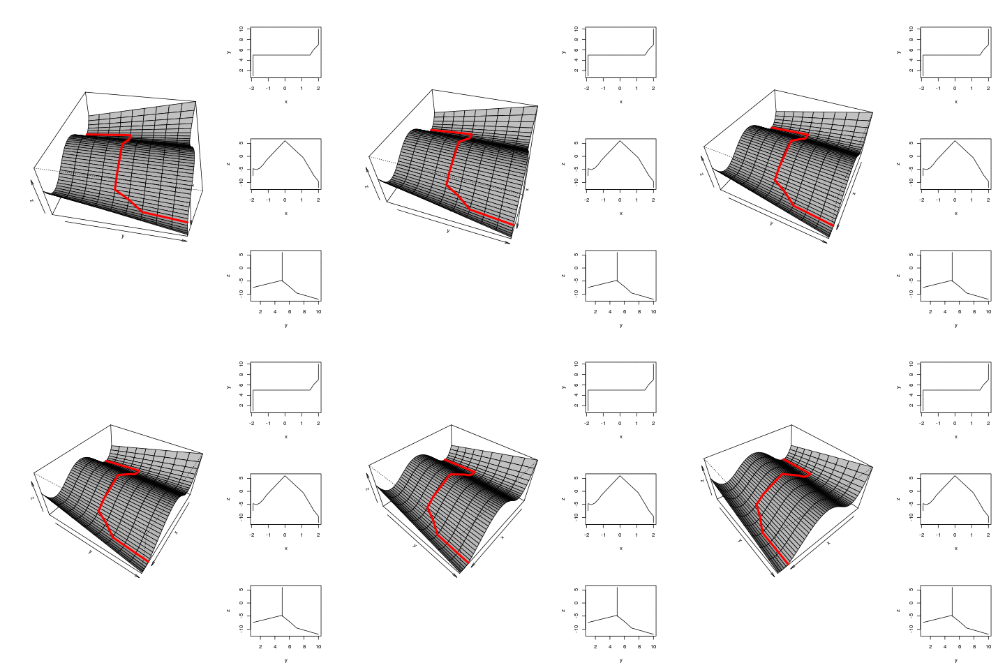
1 Try adding 2D plot of the trend overtime and the variation within basins of attraction

  • Following on from the previous work I now want to calculate the 2D paths.
  • This will then form the basis for a "walk through" animation
  • Either with recorded narration or annotations that appear at the right time to describe each transition
  • This is most of what I want to include except I have not added the wiggly variations around the main trend line, that show the system varying within the basin of attraction
  • I got advice that Blender3d was the best way to finish this off. Any other suggestions?

1.1 figure

/images/TrendsAndTriggers-v2.1.gif

1.2 code

# functions
x <- seq(from=-2.5, to=2.5, by=0.1)

# load
data_out <- read.csv("TrendsAndTriggers-v2.csv")

## do
x2d  <- matrix(NA, ncol = 3, nrow = 0)
xindex  <- c(rep(-1.9, 5), 
             -1.7, -1.5 , -1.3, -1.1, 0, 1.1, 1.3, 1.5, 1.7
             , rep(2, 4))
j  <- 1
xind  <- xindex[j]
for(index in c(1:5,rep(5,8), 6:10)){
x2d <- rbind(x2d, subset(data_out, y == index & x == xind))
j <- j + 1
xind <- xindex[j]
}
#  x2d

#png("/images/TrendsAndTriggers-v2.1.gif")
setwd("images")
saveGIF(
{
ani.options(interval = 0.2)  
for(ith in 100:140){
layout(matrix(c(1,2,1,3,1,4), 3, 2, byrow = TRUE), widths=c(2,1), heights=c(2,2,2))
# layout.show(4)
res <-  persp(x, 1:10, matrix(data_out$z, ncol = 10, nrow = length(x)),
               ylab= "y",  xlab= "x", zlab = "z",  
               theta = ith, 
               phi = 42, ltheta = 120, shade = 0.75,
               expand = 0.5, col = "lightgrey")
lines (trans3d(x2d$x, x2d$y, x2d$z, pmat = res), col = "red", lwd = 4)
plot(x2d$x, x2d$y, type = "l", xlab="x", ylab="y")
plot(x2d$x, x2d$z, type = "l", xlab="x", ylab="z")
plot(x2d$y, x2d$z, type = "l", xlab="y", ylab="z")
}
}

outdir = getwd(), movie.name = "TrendsAndTriggers-v2.1.gif"
)
setwd("..")

#  dev.off()

Posted in  ecosocial tipping points


Animation Illustrating Catastrophic Regime Shifts

Trends and Triggers Figure

Trends and Triggers Figure


1 Introduction

This work toward a enhanced figure that might be used to tell a detailed story about the mixture of trend, triggers and wiggles.

2 The History

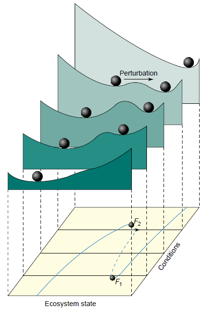
The original image I base my imagination on is:

Which was based on

  • Scheffer, M., Carpenter, S., Foley, J. a, Folke, C., & Walker, B. (2001). Catastrophic shifts in ecosystems. Nature, 413(6856), 591–6. <doi:10.1038/35098000>

/images/catastrophe.png

3 3D surface

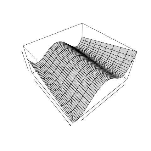
First I want to generate a 3d computer image to play with perspective and shading.

3.1 figure

/images/TrendsAndTriggers-v2.png

3.2 code

#### name:generate-surface ####
x <- seq(from=-2.5, to=2.5, by=0.1)
zid <- .1
for(y in 1:10)
{    
  z <- x^4 - zid * x^3 - 7 * x^2 + x + 6
  if(y == 1)
  {
    data_out <- cbind(x,y,z)  
  } else {
    data_out <- rbind(data_out, cbind(x,y,z))
  }
  zid <- zid + 0.1
}

data_out <- as.data.frame(data_out)
write.csv(data_out, "TrendsAndTriggers-v2.csv", row.names = F)

png("/images/TrendsAndTriggers-v2.png")
persp(x, 1:10, matrix(data_out$z, ncol = 10, nrow = length(x)), ylab= "",  xlab= "", zlab = "",  
      theta = 140, 
      phi = 42, 
      expand = 0.5, col = "lightgrey")
dev.off()

4 Try an animation

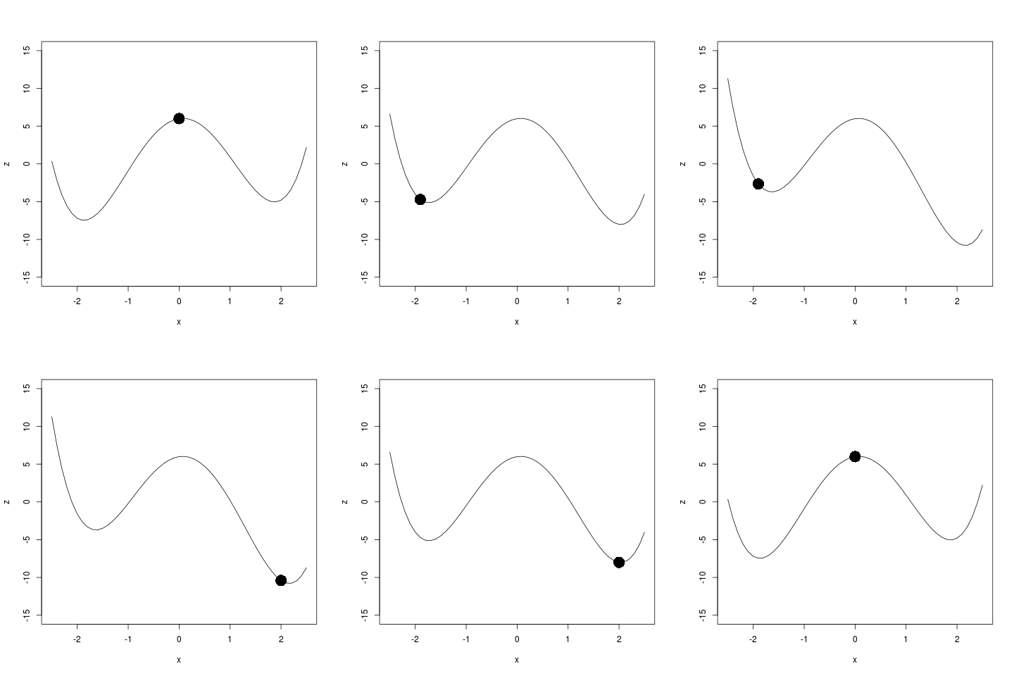
I'd like to move the ball through the surface. First need to calculate the path.

4.1 figure

/images/animation.gif

4.2 code

# functions
if(!require(animation)) install.packages("animation");
require(animation)

# load
data_out <- read.csv("TrendsAndTriggers-v2.csv")

## do
setwd("images")
saveGIF(
{
  ani.options(interval = 0.2)
  xindex  <- c(0, -1, rep(-1.9, 6), -1, 0, 1, rep(2, 6), 1, 0 , 0)
  j  <- 1
  xind  <- xindex[j]
  for(index in c(1:10, 9:1)){
  with(subset(data_out, y == index),
       plot(x, z, type = "l", ylim = c(-15,15))
       )
  with(subset(data_out, y == index & x == xind),
       points(x,z,pch=16,cex = 3)
       )
  j <- j + 1
  xind <- xindex[j]
  }
},
outdir = getwd()
)
setwd("..")

5 Next Steps

  • the polynomials should move up and down to give the height of originals
  • the hump in the middle needs to change, so the ball flips more easily
  • I'd like the ball to wiggle, add a random walk
  • the time series dimension needs to be shown
  • It'd be great to combine this with 2D line plots as well

Posted in  ecosocial tipping points