
Trends and Triggers Figure
Table of Contents
1 Introduction
This work toward a enhanced figure that might be used to tell a detailed story about the mixture of trend, triggers and wiggles.
2 The History
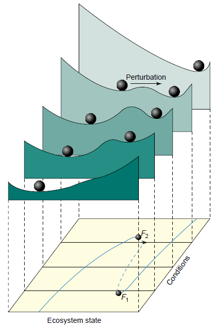
The original image I base my imagination on is:
- Scheffer, M., & Carpenter, S. R. (2003). Catastrophic regime shifts in ecosystems: linking theory to observation [Review]. TRENDS in Ecology and Evolution, 18(12), 648–656. Retrieved from http://eaton.math.rpi.edu/csums/papers/Ecostability/scheffercatastrophe.pdf
Which was based on
- Scheffer, M., Carpenter, S., Foley, J. a, Folke, C., & Walker, B. (2001). Catastrophic shifts in ecosystems. Nature, 413(6856), 591–6. <doi:10.1038/35098000>
3 3D surface
First I want to generate a 3d computer image to play with perspective and shading.
3.1 figure
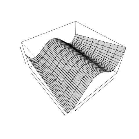
3.2 code
#### name:generate-surface ####
x <- seq(from=-2.5, to=2.5, by=0.1)
zid <- .1
for(y in 1:10)
{
  z <- x^4 - zid * x^3 - 7 * x^2 + x + 6
  if(y == 1)
  {
    data_out <- cbind(x,y,z)
  } else {
    data_out <- rbind(data_out, cbind(x,y,z))
  }
  zid <- zid + 0.1
}

data_out <- as.data.frame(data_out)
write.csv(data_out, "TrendsAndTriggers-v2.csv", row.names = F)

png("/images/TrendsAndTriggers-v2.png")
persp(x, 1:10, matrix(data_out$z, ncol = 10, nrow = length(x)), ylab= "",  xlab= "", zlab = "",
      theta = 140,
      phi = 42,
      expand = 0.5, col = "lightgrey")
dev.off()
4 Try an animation
I'd like to move the ball through the surface. First need to calculate the path.
4.1 figure
4.2 code
# functions
if(!require(animation)) install.packages("animation");
require(animation)

# load
data_out <- read.csv("TrendsAndTriggers-v2.csv")

## do
setwd("images")
saveGIF(
{
  ani.options(interval = 0.2)
  xindex  <- c(0, -1, rep(-1.9, 6), -1, 0, 1, rep(2, 6), 1, 0 , 0)
  j  <- 1
  xind  <- xindex[j]
  for(index in c(1:10, 9:1)){
  with(subset(data_out, y == index),
       plot(x, z, type = "l", ylim = c(-15,15))
       )
  with(subset(data_out, y == index & x == xind),
       points(x,z,pch=16,cex = 3)
       )
  j <- j + 1
  xind <- xindex[j]
  }
},
outdir = getwd()
)
setwd("..")
5 Next Steps
- the polynomials should move up and down to give the height of originals
- the hump in the middle needs to change, so the ball flips more easily
- I'd like the ball to wiggle, add a random walk
- the time series dimension needs to be shown
- It'd be great to combine this with 2D line plots as well


