Welcome to my Open Notebook

This is an Open Notebook with Selected Content - Delayed. All content is licenced with CC-BY. Find out more Here.

ONS-SCD.png

Decisions to make when modelling interactions

This post focuses on decision making during statistical modelling. The case of investigating effect modification is used as an example. The analyst has several options available to them when constructing the model parametrisation for adjustment to explain modification effectively. Unlike confounding (in which the criterion of substantial magnitude change of the effect estimate when controlling for a third variable can be easily assessed), models including effect modification can be hard to interpret. Taking account of effect modification becomes increasingly important when modelling complex interactions.

If an effect moderator is present then the relationship between exposure and response varies between different levels of the moderator. An example is provided by a paper we published, in which the relationship between proximity to wetlands and Ross River virus infection was found to be different for towns and rural areas, where the ‘urban’ variable is the ‘effect moderator’.

There are three common ways for data analysts to address this question in statistical models:

  1. multiple models for each group,
  2. interaction terms or
  3. re-parametrisation to explicitly depict interactions.

The first way is to split apart the dataset and conduct separate analyses of multiple groups. For example, one could run the regression in the urban zone and the rural zone seperately and see if there were different exposure response functions in the two models. This was the approach of our paper. This approach has the strength that it is simple to do and yeilds results that are easy to interpret. A limitation of this method is that by splitting the dataset one loses degrees of freedom and therefore statistical power.

The second approach (which removes that limitation of the first option) is to fit interaction terms. The example shown in Figure 1 is a multiplicative interaction model (Brambor 2006). This approach was not taken in the models reported in our paper, but can easily be implemented and shows that the function of distance was estimated to have different ‘slopes’ in each of the dichotomous urban groups.

The statistical method can be easily implemented in software by including a multiplicative term between two variables, however in practice the resulting post estimation regression outputs can be difficult to interpret. For example, say one wants to calculate the effect and standard error for exposure X on health outcome Y with the interaction of the effect modifier Z. The form of this model can be written as:

\[Y ~ \beta_{1}X + \beta_{2}Z + \beta_{3}XZ\]

where B1, B2 and B3 are the regression coefficients estimated and the term XZ is the interaction between exposure and effect modifier.

The difficulty for interpretation comes when using this method for calculating the marginal effect of X on Y and the conditional standard error. The specific method described in Brambor et al. is:

  1. Calculate the coefficients and the variance-covariance matrix from the regression model
  2. The marginal effect is $\beta_{1} + \beta_{3}XZ$ where Z is the level of the modifying factor (0 or 1 in the dichotomous effect modifier case)
  3. The conditional standard error is:
\[\sqrt{var(\beta_{1}) + Z^2 var(\beta_{3}) + 2Zcov(\beta_{1}\beta_{3})}\]

Therefore the strengths of this approach is that it does not reduce degrees of freedom and is straightforward to specify the model in standard statistical software packages. The limitations are related to interpretation of the resulting coefficients for both the main effects and the marginal effects, and standard errors for these.

The third approach available to analysts makes it easier to access the resulting regression output. This method was employed in Paper 1 in the final modelling phase in which estimates were calculated for the different drought exposure-response funcitons in each of the sub-groups. In the terms of Figure \ref{fig:effectmod.png} it is simple to:

  1. Calculate X1 = X * Z (i.e = exposure for condition is met, zero otherwise)
  2. Calculate X0 = X * (1-Z) (i.e. = exposure for NON-condition, zero for condition is TRUE)
  3. Instead of X, Z and XZ, fit X1, X0 and Z. This model also contains three parameters and captures the same interactions as it is the same model with a different parametrisation. The standard errors for the X1 and X0 are calculated directly from the regression.

This method is much easier to implement and interpret. This is also considerably more flexible than the other two approaches. A limitation remains for this method in that the pre-processing steps required are more complicated, and there are inherently more possibilities for the data analyst to make errors in writing their code as they make these changes to the analytical data.

# Demonstrating this with the data from the paper (available in table 2)
## the following code shows the different parametrisations for the effect modification by urban
## we show that the coeffs and se are equivalent but that the psuedo-R
## squared will be better when including all our data in stratified analysis

# model 0 effect in eastern
d_eastern
fit <- glm(cases~ buffer + offset(log(1+pops)),family='poisson', data=d_eastern )
summa <- summary(fit)
summa
## Coefficients:
##             Estimate Std. Error z value Pr(>|z|)
## (Intercept) -4.82425    0.14451 -33.382  < 2e-16 ***
## buffer      -0.24702    0.07921  -3.119  0.00182 **

# model 1 effect in urban
fit1 <- glm(cases~ buffer + offset(log(1+pops)),family='poisson', data=d_urban )
summa <- summary(fit1)
summa
## Coefficients:
##             Estimate Std. Error z value Pr(>|z|)
## (Intercept) -5.52363    0.33354 -16.561   <2e-16 ***
## buffer       0.03853    0.06352   0.607    0.544

# step 1, combine the urban and rural data
d_eastern$urban <- 0
d_urban$urban <- 1
dat2 <- rbind(d_eastern, d_urban)
str(dat2)
dat2

# model 2 is a multiplicative term
fit2 <- glm(cases ~ buffer * urban + offset(log(1+pops)), family = 'poisson', data = dat2)
summa <- summary(fit2)
summa
## Coefficients:
##              Estimate Std. Error z value Pr(>|z|)
## (Intercept)  -4.82425    0.14451 -33.382  < 2e-16 ***
## buffer       -0.24702    0.07921  -3.119  0.00182 **
## urban        -0.69938    0.36350  -1.924  0.05435 .
## buffer:urban  0.28555    0.10153   2.812  0.00492 **

# the coeff on buffer is for urban = 0 is main effect
# the coeff on buffer:urban is for urban = 1 is the marginal effect
b1 <- summa$coeff[2,1]
b3 <- summa$coeff[4,1]
b1 + b3
# 0.0385268
# but what about that p-value?  and the se?
str(fit2)
fit2_vcov <- vcov(fit2)
fit2_vcov
# now calculate the conditional standard error for the marginal effect of buffer for the value of the modifying variable (Z, urban =1)
varb1<-fit2_vcov[2,2]
varb3<-fit2_vcov[4,4]
covarb1b3<-fit2_vcov[2,4]
Z<-1
conditional_se <- sqrt(varb1+varb3*(Z^2)+2*Z*covarb1b3)
conditional_se


# model 3 is the re-parametrisation
dat2$buffer_urban <- dat2$buffer * dat2$urban
dat2$buffer_eastern <- dat2$buffer * (1-dat2$urban)

fit3 <- glm(cases ~ buffer_urban + buffer_eastern + urban + offset(log(1+pops)), family = 'poisson', data = dat2)
summa <- summary(fit3)
summa

## Coefficients:
##                Estimate Std. Error z value Pr(>|z|)
## (Intercept)    -4.82425    0.14451 -33.382  < 2e-16 ***
## buffer_urban    0.03853    0.06352   0.607  0.54416
## buffer_eastern -0.24702    0.07921  -3.119  0.00182 **
## urban          -0.69938    0.36350  -1.924  0.05435 .

Posted in  disentangle statistical modelling


Show missingness in large dataframes, version 2

The old post

/images/bankstown_traffic_counts_full_listing_june_2014.svg

Code

misstable <- function(atable){
 op <- par(bg = "white")
 plot(c(0, 400), c(0, 1000), type = "n", xlab="", ylab="",
     main = "Missing Data Table")


 pmin=000
 pmax=400
 stre=pmax-pmin
 lnames=length(atable)
 cstep = (stre/lnames)
 for(titles in 1:lnames){
 text((titles-1) * cstep+pmin+cstep/2,1000,colnames(atable)[titles])
 }

 gmax=900
 gmin=0
 gstre=gmax-gmin
 rvec = as.vector(atable[ [ 1 ] ])
 dnames=length(rvec)
 step = gstre / dnames
 for(rows in 1:dnames){
 text(30,gmax - (rows-1)*step-step/2,rvec[rows])
 ymax=gmax - (rows-1)*step
 ymin=gmax - (rows)*step
 for(col in 2:lnames-1){
 if(atable[rows,col+1] == F){
 tcolor = "red"
 }
 if(atable[rows,col+1] == T){
 tcolor = "white"
 }
 rect((col) * (stre/lnames)+pmin, ymin, (col+1) * (stre/lnames)+pmin,
 ymax,col=tcolor,lty="blank")
 }
 }
}

  • Now things to note are that the function expects the data to be TRUE if Not NA and FALSE if is NA
  • so might need to massage things a bit first
  • here is the small test Grant supplied

Code

require(grDevices)
   
# Make a quick dataframe with true/false representing data availability
locs=c("Australia","India","New Zealand","Sri Lanka","Uruguay","Somalia")
f1=c(T,F,T,T,F,F)
f2=c(F,F,F,T,F,F)
f3=c(F,T,T,T,F,T)
atable=data.frame(locs,f1,f2,f3)
atable
#Draw the table.
misstable(atable)

  • here is the one I worked on today

Code

# having defined the input dir and input file tried reading the excel sheet (without head 3 rows)
#dat <- readxl::read_excel(file.path(indir, infile), skip =3)
# got lots of warnings()
## 50: In read_xlsx_(path, sheet, col_names = col_names, col_types = col_types,  ... :
##   [1278, 4]: expecting date: got '[NULL]'
# I always worry about using excel connections so open in excel (in windows) 
# and save as to convert to CSV
dat <- read.csv(file.path(indir, gsub(".xlsx", ".csv", infile)), skip =3, stringsAsFactor = F)
str(dat)
# 'data.frame':     1396 obs. of  167 variables:
# but most of the cols and a third of the rows are empty!
# check missings
dat2 <- data.frame(id = 1:nrow(dat), dat)
str(dat2)
# first if they are empty strings
dat2[dat2 == ""] <- NA
# now if NA
dat2[,2:ncol(dat2)] <- !is.na(dat2[,2:ncol(dat2)])

# Truncate the hundreds of empty cols
str(dat2[,1:18])
tail(dat2[,1:18])
svg(file.path(outdir, gsub(".csv", ".svg", outfile))    )
misstable(dat2[,1:18])
dev.off()
browseURL(file.path(outdir, gsub(".csv", ".svg", outfile))    )

# cool, that is an effective way to look at the data

Posted in  disentangle Exploratory Data Analysis


show-missingness-in-large-dataframes

Sometime ago I saw this example of a method for assessing missing data in a large data frame http://flowingdata.com/2014/08/14/csv-fingerprint-spot-errors-in-your-data-at-a-glance/

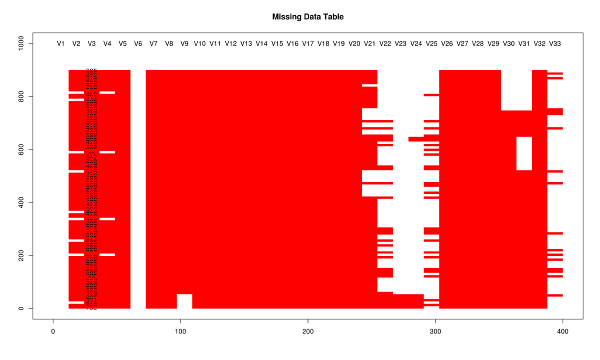
I asked my colleague Grant about doing this in R and he whipped up the following code to generate such an image:

/images/misstable.png

Code

misstable <- function(atable){
 op <- par(bg = "white")
 plot(c(0, 400), c(0, 1000), type = "n", xlab="", ylab="",
     main = "Missing Data Table")


 pmin=000
 pmax=400
 stre=pmax-pmin
 lnames=length(atable)
 cstep = (stre/lnames)
 for(titles in 1:lnames){
 text((titles-1) * cstep+pmin+cstep/2,1000,colnames(atable)[titles])
 }

 gmax=900
 gmin=0
 gstre=gmax-gmin
 rvec = as.vector(atable[ [ 1 ] ])
 dnames=length(rvec)
 step = gstre / dnames
 for(rows in 1:dnames){
 text(30,gmax - (rows-1)*step-step/2,rvec[rows])
 ymax=gmax - (rows-1)*step
 ymin=gmax - (rows)*step
 for(col in 2:lnames-1){
 if(atable[rows,col+1] == F){
 tcolor = "red"
 }
 if(atable[rows,col+1] == T){
 tcolor = "white"
 }
 rect((col) * (stre/lnames)+pmin, ymin, (col+1) * (stre/lnames)+pmin,
 ymax,col=tcolor,lty="blank")
 }
 }
}

require(grDevices)
   
# Make a quick dataframe with true/false representing data availability
locs=c("Australia","India","New Zealand","Sri Lanka","Uruguay","Somalia")
f1=c(T,F,T,T,F,F)
f2=c(F,F,F,T,F,F)
f3=c(F,T,T,T,F,T)
atable=data.frame(locs,f1,f2,f3)
atable
#Draw the table.
misstable(atable)

Posted in  disentangle Exploratory Data Analysis


Sanitize mendeley references in r markdown reporting

A key challenge for Reproducible Research Reports in Rmarkdown remains adequate scholarly citation management; the machinery of scholarly citations and references.

The knitcitations R package does a great job of working with bibtex bibliography files, however the bibtex manager that I use is Mendeley and it has implemented some rules on the way it handles special characters that forces the bibtex references into a state with some ‘escaped’ elements that breaks their presentation via knitcitations.

This is a post from my open notebook that shows the workaround I am using for sanitizing the Mendeley escaped underscores in URLS.

Here is an example:

There is considerable public health impact from the effects on mental of drought (Sarathi Biswas 2012). It is proposed that the best method to disentangle the multifactorial nature of this causal mechanism is the ‘five-capitals’ framework, indeed this method may even enable understanding the human carrying capacity of ecosystems (McMichael & Butler 2002).

McMichael, A.J. & Butler, C.D. (2002). Global health trends: Evidence for and against sustainable progress. International Union for the Scientific Study of Population Committee on Emerging Health Threats. http://www.demogr.mpg.de/papers/workshops/020619{\_}paper25.pdf [21 Sep. 2003]

Sarathi Biswas, P. (2012). Alcohol, drought lead to farmer’s suicide. Daily News and Analysis. http://www.dnaindia.com/pune/report{\_}alcohol-drought-lead-to-farmers-suicide{\_}1688976 [17 May 2012]

See those pesky curly braces { and } around the underscores?

The fix

The fix I am using is to sanitize each record where this is an issue as I build my document, so the mendeley version stays as-is, while the R version has been sanitized by removing the escape characters.

# read mendeley bibtex file
bib <- read.bibtex("~/references/library.bib")
# ad hoc fix
for(bibkey in c("SarathiBiswas2012", "Mcmichael2002a")){
  bib[ [ bibkey ] ]$url <- gsub("\\{\\\\_\\}","_", bib[ [ bibkey ] ]$url)
}

This is the result:

McMichael, A.J. & Butler, C.D. (2002). Global health trends: Evidence for and against sustainable progress. International Union for the Scientific Study of Population Committee on Emerging Health Threats. http://www.demogr.mpg.de/papers/workshops/020619_paper25.pdf [21 Sep. 2003]

Sarathi Biswas, P. (2012). Alcohol, drought lead to farmer’s suicide. Daily News and Analysis. http://www.dnaindia.com/pune/report_alcohol-drought-lead-to-farmers-suicide_1688976 [17 May 2012]

Posted in  disentangle Reproducible Research Reports


Keeping an electronic lab notebook for computational statistics projects

  • In my previous post on this topic http://ivanhanigan.github.io/2015/10/how-to-effectively-implement-electronic-lab-notebooks-in-epidemiology/ I summarised some recommendations for electronic lab notebooks
  • I’ve collated from a variety of sources for managing computational statistics projects in a reproducible research Pipelines
  • One thing I found while reading the literature around this topic is that the concepts are difficult to really grasp until I see them being used
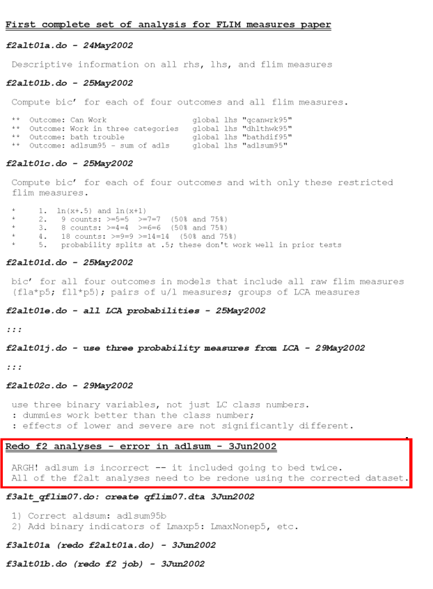
  • The example worklog from Scott Long was a good insight into his method, that I really got more out of the figure below than from descriptions of the concept
  • screen shot taken from Long, S. (2012). Principles of Workflow in Data Analysis. Retrieved from http://www.indiana.edu/~wim/docs/2012-long-slides.pdf (accessed 2015-10-23).

/images/worklog-long.png

  • I added a red box around an important aspect of this example, the communication of gory details, that are often difficult to track if not using a notebook to log our work
  • ARGH! indeed.

Replication from Noble’s description

  • That looks good, but I also really liked the description in Noble’s paper where scripts that do computations are linked to log entries
  • This was something that I felt I wanted to see in action
  • Without an example online, I had to have a go at creating one from the instructions
  • I also had to make some modifications to the method because I want to have this set up work in a multidisciplinary team with some users on windows and others on linux, sharing the project on a network folder

My paraphrasing of Noble’s description

  • Worklog: this is the main file, like a ‘lab notebook’ for the analyst to track their work. This document resides in the root of the project directory and records your progress in detail. Entries in the notebook should be dated, and they should be relatively verbose, with links or embedded images or tables displaying the results of the experiments that you performed. In addition to describing precisely what you did, the notebook should record your observations, conclusions, and ideas for future work
  • For group work, this can also contain a ‘working’ folder for each person to store their messy day-to-day files that we don’t want to clutter up the main folder (eg ‘working_ivan’)

Conventions I used for writing the worklog entries are:

  • Names follow this structure [**] [date in ISO 8601 YYYY-MM-DD] [meeting/notes/results] [with/from UserName] [Re: topic shortname]
  • ‘meetings’ are for both agenda preparation and also notes of discussion
  • ‘notes’ are such things as emailed information or ad hoc Discovery
  • ‘results’ are entries related to a section of the ‘results’ folder. That is, this kind of entry is in parallel to the results entry (see below), however the log contains a prose description of the experiment, whereas the results folder contains scripts etc of all the gory details.

Tests

  • I use Emacs on linux for most of my work but I need to share with windows users so tested out keeping the log in a MS word doc. This got corrupted quickly I think because I edited in Libre office.
  • I decided to try and just use a plain text format
  • text files created in Ubuntu are so difficult to understand (read) when opened in Windows’ Notepad. No matter how many lines have been used, all the lines appear in the same one line. To set the buffer coding to DOS style issue:

M-x set-buffer-file-coding-system utf-8-dos

a couple of examples

  • As this is a plain text document opening it in emacs will not automatically render it in the Orgmode fashion
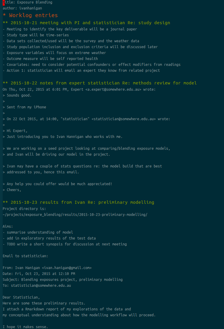
  • To achieve this the command is M-x org-mode and the file looks like below

/images/worklog-ivan1.png

  • From here I can keep adding new entries at the bottom, and have a section for URGENT ACTION a the top
  • Orgmode can expand the entries by moving to that line and hitting TAB, or use the command C-u C-u C-u TAB to expand all branches

/images/worklog-ivan2.png

the ‘Experiment Results’ level is about work you might do on a single day, or over a week or two

  • Each results subfolder would have workflow scripts that does the work
  • At this level each ‘experiment’ is written up in chronological order
  • It is recommended to store every command used while performing the experiment preferably as an executable script that carries out the entire experiment automatically
  • you should end up with a file that is parallel to the worklog entry
  • The worklog contains a prose description of the experiment, whereas the driver script contains all the gory details
  • this is the level I usually think of the distribution side of things
  • You may want to pack up the results from one of these folders and email it to the collaborators, or decide on the one set of tables and figures to write into the manuscript for submission to a journal
  • If this is accepted for publication, this is the one combined package of ‘analytical data and code’ that I would consider putting up online as supporting information for the paper.

Example

  • I followed Noble’s advice to create a driver script to set up the folder structure:
  • it is in my Github R package disentangle
> dir.create("exposures_blending")
> setwd("exposures_blending")
> disentangle::AdminTemplate()
[1] TRUE
> dir.create("results")
> setwd("results")
> makeProject::makeProject("2015-10-23-preliminary-modelling")
Creating Directories ...
Creating Code Files ...
Complete ...
> 

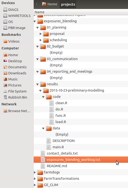
This populates the folders as shown below

/images/worklog-ivan3.png

Conclusions

  • I feel pretty happy with this as a replication of Noble’s method
  • My colleagues can look at my work and see a high level log that links to the gory details of day to day life in the trenches
  • The only downside I can see at the moment is that my colleagues on windows will see a text file that is pretty dense, and will not be as easy to navigate as a word document (or emacs org file)
  • Perhaps notepad++ can be used instead. On my windows machine I did a quick experiment with NPP and found that under the Language menu > Define your language there is a method to define code folding with ** as the opening. Just need to define a closing tag. I experimented with ‘—’ which might be good, but ultimately I don’t think my colleagues are going to want to do this on their machines.

Posted in  disentangle Workflow tools