• In my previous post on this topic http://ivanhanigan.github.io/2015/10/how-to-effectively-implement-electronic-lab-notebooks-in-epidemiology/ I summarised some recommendations for electronic lab notebooks
• I’ve collated from a variety of sources for managing computational statistics projects in a reproducible research Pipelines
• One thing I found while reading the literature around this topic is that the concepts are difficult to really grasp until I see them being used
• The example worklog from Scott Long was a good insight into his method, that I really got more out of the figure below than from descriptions of the concept
• screen shot taken from Long, S. (2012). Principles of Workflow in Data Analysis. Retrieved from http://www.indiana.edu/~wim/docs/2012-long-slides.pdf (accessed 2015-10-23).

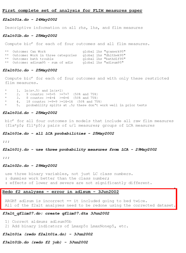
• I added a red box around an important aspect of this example, the communication of gory details, that are often difficult to track if not using a notebook to log our work
• ARGH! indeed.

Replication from Noble’s description

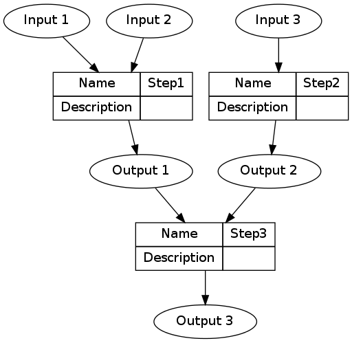
• That looks good, but I also really liked the description in Noble’s paper where scripts that do computations are linked to log entries
• This was something that I felt I wanted to see in action
• Without an example online, I had to have a go at creating one from the instructions
• I also had to make some modifications to the method because I want to have this set up work in a multidisciplinary team with some users on windows and others on linux, sharing the project on a network folder

My paraphrasing of Noble’s description

• Worklog: this is the main file, like a ‘lab notebook’ for the analyst to track their work. This document resides in the root of the project directory and records your progress in detail. Entries in the notebook should be dated, and they should be relatively verbose, with links or embedded images or tables displaying the results of the experiments that you performed. In addition to describing precisely what you did, the notebook should record your observations, conclusions, and ideas for future work
• For group work, this can also contain a ‘working’ folder for each person to store their messy day-to-day files that we don’t want to clutter up the main folder (eg ‘working_ivan’)

Conventions I used for writing the worklog entries are:

• Names follow this structure [**] [date in ISO 8601 YYYY-MM-DD] [meeting/notes/results] [with/from UserName] [Re: topic shortname]
• ‘meetings’ are for both agenda preparation and also notes of discussion
• ‘notes’ are such things as emailed information or ad hoc Discovery
• ‘results’ are entries related to a section of the ‘results’ folder. That is, this kind of entry is in parallel to the results entry (see below), however the log contains a prose description of the experiment, whereas the results folder contains scripts etc of all the gory details.

Tests

• I use Emacs on linux for most of my work but I need to share with windows users so tested out keeping the log in a MS word doc. This got corrupted quickly I think because I edited in Libre office.
• I decided to try and just use a plain text format
• text files created in Ubuntu are so difficult to understand (read) when opened in Windows’ Notepad. No matter how many lines have been used, all the lines appear in the same one line. To set the buffer coding to DOS style issue:

M-x set-buffer-file-coding-system utf-8-dos

a couple of examples

• As this is a plain text document opening it in emacs will not automatically render it in the Orgmode fashion
• To achieve this the command is M-x org-mode and the file looks like below

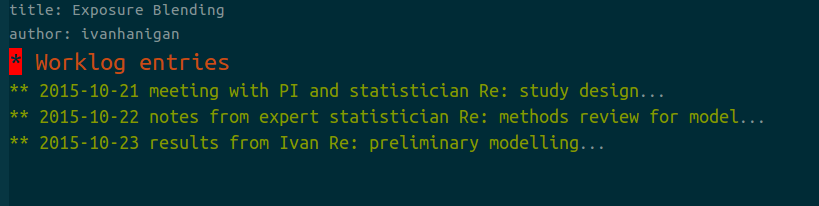
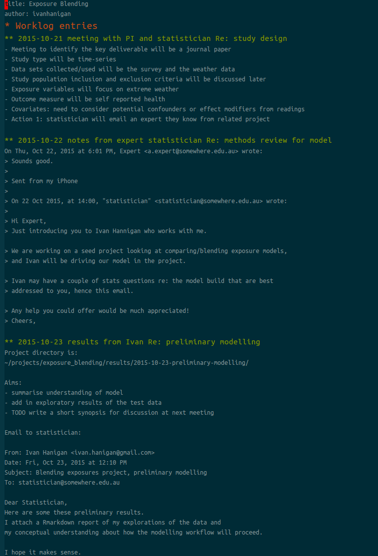
• From here I can keep adding new entries at the bottom, and have a section for URGENT ACTION a the top
• Orgmode can expand the entries by moving to that line and hitting TAB, or use the command C-u C-u C-u TAB to expand all branches

the ‘Experiment Results’ level is about work you might do on a single day, or over a week or two

• Each results subfolder would have workflow scripts that does the work
• At this level each ‘experiment’ is written up in chronological order
• It is recommended to store every command used while performing the experiment preferably as an executable script that carries out the entire experiment automatically
• you should end up with a file that is parallel to the worklog entry
• The worklog contains a prose description of the experiment, whereas the driver script contains all the gory details
• this is the level I usually think of the distribution side of things
• You may want to pack up the results from one of these folders and email it to the collaborators, or decide on the one set of tables and figures to write into the manuscript for submission to a journal
• If this is accepted for publication, this is the one combined package of ‘analytical data and code’ that I would consider putting up online as supporting information for the paper.

Example

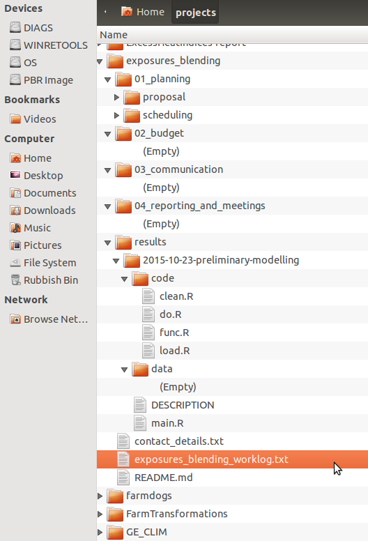
• I followed Noble’s advice to create a driver script to set up the folder structure:
• it is in my Github R package disentangle

> dir.create("exposures_blending")
> setwd("exposures_blending")
> disentangle::AdminTemplate()
[1] TRUE
> dir.create("results")
> setwd("results")
> makeProject::makeProject("2015-10-23-preliminary-modelling")
Creating Directories ...
Creating Code Files ...
Complete ...
> 

This populates the folders as shown below

Conclusions

• I feel pretty happy with this as a replication of Noble’s method
• My colleagues can look at my work and see a high level log that links to the gory details of day to day life in the trenches
• The only downside I can see at the moment is that my colleagues on windows will see a text file that is pretty dense, and will not be as easy to navigate as a word document (or emacs org file)
• Perhaps notepad++ can be used instead. On my windows machine I did a quick experiment with NPP and found that under the Language menu > Define your language there is a method to define code folding with ** as the opening. Just need to define a closing tag. I experimented with ‘—’ which might be good, but ultimately I don’t think my colleagues are going to want to do this on their machines.

Adequately documenting the methods and results of data analysis helps safeguard against errors of execution and interpretation. It is proposed that reproducible research pipelines address the problem of adequate documentation of data analysis.

This is because they make it easy to check the methods. Assumptions are easy to challenge and results verified in new analyses. Reproducible research pipelines extend traditional research. They do this by encoding the steps in a computer ‘scripting’ language and distributing the data and code with publications. Traditional research moves through the steps of hypothesis and design, measured data, analytic data, computational results (for figures, tables and numerical results), and reports (text and formatted manuscript).

Fundamental components of a reproducible research pipeline

The basic components of a pipeline are:

• Data Management Plan and Data Inventory
• Method steps
• Code
• Data storage
• Reports
• Distribution.

Method Steps

The method step is the key atomic unit of a scientific pipeline. It consists of inputs, outputs and a rationale for why the step is taken.

A simple way to keep track of the steps, inputs and outputs is shown in the Table below.

library(stringr)
steps <- read.csv(textConnection('
CLUSTER ,  STEP  , INPUTS                   , OUTPUTS                   
A  ,  Step1      , "Input 1, Input 2"       , "Output 1"                 
A  ,  Step2      ,  Input 3                  , Output 2                   
B  ,  Step3      , "Output 1, Output 2"      , Output 3                  
'), stringsAsFactors = F, strip.white = T)

The steps and data listed in the Table above can be visualised. To achieve this an R function was written as part of this PhD project and is distributed in my own R package available on Github https://github.com/ivanhanigan/disentangle. This is the newnode function. The function returns a string of text written in the dot language which can be rendered in R using the DiagrammeR package, or the standalone graphviz package. This creates the graph of this pipeline shown in Figure below. Note that a new field was added for Descriptions as these are highly recommended.

library(disentangle); library(stringr)
nodes <- newnode(indat = steps,   names_col = "STEP", in_col = "INPUTS",
  out_col = "OUTPUTS", 
  nchar_to_snip = 40)
sink("fig-basic.dot");
cat(nodes);
sink()
# or DiagrammeR::grViz(nodes)
system("dot -Tpdf fig-basic.dot -o fig-basic.pdf")

• It is often stated in the literature that an electronic lab notebook is a core component of reproducible research
• For example the following is from Buck, S. (2015). Solving reproducibility. Science, 348(6242), 1403–1403. http://dx.doi.org/10.1126/science.aac8041

one of the most effective ways to promote high-quality science 
is to create free open-source tools that give scientists
easier and cheaper ways to incorporate transparency
into their daily workflow: from open lab notebooks, to
software that tracks every version of a data set, to dynamic 
document generation.

• But I have struggled to operationalise the lab notebook in the epidemiology projects I work in
• Here are some notes based on my recent readings and attempts with a new team

Modularised lab notebooks

There seem to be a small number of components to a lab notebook that can be defined as:

• Data management plan
• Workplan
• Worklog
• Workflow
• Distribution

One thing I think is important is to have levels of organisation in a hierarchy:

• Macro level: The ‘Research Programme’ level is about the entire breadth of the projects in the group.
  • Data Management Plan: including managing the computers and a Data Inventory
  • Personal Workplan and Worklog: this is an overview of things I do, plan to do or learn along the way (this is for the high level things like planning professional development, or a holiday)
  • This is operationalised in the blog you are reading right now.
• Meso level: the ‘Research Project’ level is about a single study, or a small group of studies based around a core dataset or Concept
  • This is the level that you might write up a manuscript for a journal, or report to a client
  • Project workplan: at this level there may be high level information about the study design, hypotheses, resources and admin for managing relationships with a variety of collaborators
  • Worklog: WS Noble http://dx.doi.org/10.1371/journal.pcbi.1000424 recommends that this be the main lab notebook for the analysts
  • He says ‘This is a document that resides in the root of the results directory and that records your progress in detail. Entries in the notebook should be dated, and they should be relatively verbose, with links or embedded images or tables displaying the results of the experiments that you performed. In addition to de- scribing precisely what you did, the notebook should record your observations, conclusions, and ideas for future work’
• Micro level: the ‘Experiment Results’ level is about work you might do on a single day, or over a week
  • Workflow scripts: At this level each ‘experiment’ is written up in chronological order, as entries to the Worklog at the meso level
  • Noble recommends ‘create either a README file, in which I store every command line that I used while performing the experi- ment, or a driver script (I usually call this runall) that carries out the entire experiment automatically’…
  • and ‘you should end up with a file that is parallel to the lab notebook entry. The lab notebook contains a prose description of the exper- iment, whereas the driver script contains all the gory details.’
  • this is the level I usually think of managing the distribution side of things. I will want to pack up the results and email to my collaborators, or decide on the one set of tables and figures to write into the manuscript for submission to a journal. If this is accepted for publication, this is the one combined package of ‘analytical data and code’ that I would consider putting up online (to github) as supporting information for the paper.

• I have been using RGDAL to transform and write out spatial data in GDA94
• It is a problem to know what I need to do to create the right prj file for ArcGIS to read without complaining
• I have an example of code below, that I used on a dataset I knew was in GDA94 when I read it in. I want to do this mostly for when I have to convert from one to another, but I have done the manual hack a couple of times now and thought I better just check with an expert.

R Code:

infile <- "ap_map"
outfile <- gsub("map", "map_GDA94.shp", infile)
outfile
setwd(indir)
shp <- readOGR(".", infile)
setwd(projdir)
plot(shp, add = T)
#str(shp)
shp@proj4string@projargs
#[1] "+proj=longlat +ellps=GRS80 +no_defs"
# confirm this is GDA94
epsg <- make_EPSG()
str(epsg)
epsg[grep(4283, epsg$code),]
#     code    note                                                       prj4
# 212 4283 # GDA94   +proj=longlat +ellps=GRS80 +towgs84=0,0,0,0,0,0,0 +no_defs
# Arcmap sees this as GRS 1980(IUGG, 1980) which I think is the same thing
# to be on the safe side I will force it to refer to GDA94
shp2 <- spTransform(shp, CRS("+init=epsg:4283"))
shp2@proj4string@projargs
#now write
setwd(outdir)
dir()
writeOGR(shp2,  outfile, gsub(".shp", "", outfile), driver = "ESRI Shapefile")
setwd(projdir)
# Checking this shows it did not write the correct prj file, but I believe that this is because the GDA94 definition is not different to the WGS80 params.
# one other option is to manually replace that prj file with the correct text found at http://spatialreference.org/ref/epsg/4283/
# SO I did this to avoid any future confusions
# OLD GEOGCS["GRS 1980(IUGG, 1980)",DATUM["D_unknown",SPHEROID["GRS80",6378137,298.257222101]],PRIMEM["Greenwich",0],UNIT["Degree",0.017453292519943295]]
# NEW GEOGCS["GDA94",DATUM["D_GDA_1994",SPHEROID["GRS_1980",6378137,298.257222101]],PRIMEM["Greenwich",0],UNIT["Degree",0.017453292519943295]]
# checked with ArcMap and they align ok

I asked on of my colleagues and here is his reply

• I usually use the sp and maptools library, rather than the readOGR and writeOGR functions. Generally my workflow, as an example of projecting a GDA94 zone 55 file to WGS84, would be something like:

R Code:

shp <- readShapePoly("myfile.shp")
proj4string(shp) <- "+proj=utm +zone=55 +south +ellps=GRS80 +towgs84=0,0,0,0,0,0,0 +units=m +no_defs"
shp2 <- spTransform(shp, CRS("+proj=longlat +ellps=WGS84 +datum=WGS84 +no_defs "))
writePolyShape(shp2,"myfile_p.shp",proj4string=CRS("+proj=longlat +ellps=WGS84 +datum=WGS84 +no_defs "))

• I’ve never noticed any problems doing this, the projection file is generated and I’ve never noticed any alignment problems in ArcMap. It’s true that I recall ArcMap sometimes displays an incorrect plaintext projection description, but things seem to be in the right place.

• Also, I don’t really ever rely on EPSG numbers in R - I just grab the proj4 strings and try to use them directly.

TODO, see if PostGIS handles this OK

• I wonder if my FOSS GIS stack should still pass things through PostGIS as I suspect it does these things better.
• I might check the output if I run it through the DB use st_transform and then extract to shapefile.

The New York Times ran a piece on August 17, 2014: “For Big-Data Scientists, ‘Janitor Work’ Is Key Hurdle to Insights” [1]. The article bemoaned the need for too much of what data scientists call “data wrangling”, “data munging” and “data janitor work”. In essence this means data quality control processes. A key task of my role as data manager/analyst is to perform Exploratory Data Analysis (EDA) to review data deposited for consistency, quality and its compliance with standards to ensure that reusability of data published in the portal is maximised. To do this, I use relevant data formatting standards (for example the International Standards from ISO), undertake thorough taxonomic reviews of each dataset and have well documented procedures for dealing with miscellaneous errors such as data inconsistencies, duplicate variable names and reformatting numeric or character strings. I sometimes make changes to the data and give no further thoughts to it, but at other times I need to make recommendations to the data provider and ask for their decisions/approvals on what to change.

I have put down this set of guidelines for my procedures to create standardised data structures, based on things that have been recommended in the literature [2-6] to make data as re-usable as possible. Here is a list of standard amendments undertaken during my EDA process:

• identify any out-of-range values (based on the specified units), or questionable data in general;
• rename all files and variables using lower_case_with_underscores naming convention;
• tabulate frequencies and variable distributions, note any outliers for review;
• identify any opportunities to make wide data longer, or many files that can be merged;
• If you have multiple linked tables, each table should include a column that allows those tables to be linked unambiguously (such as the site_ID variables); check that linking variables that link two or more data tables are identical in each table
• check that values in linked files marry up to values in other files (eg a site code in one file that is missing from the spatial data file);
• write as CSV with quote encapsulated strings (for archival purposes);
• code missing data as NA, or identify if these were actually censored;
• coerce dates to ISO 8601 to be in the the YYYY-MM-DD format, or MMM-YYYY;
• cast nominal variables that use integer codes as character;
• check that all value labels in enumerated lists are described (ie codes for “1” = “low”, “2” = “mid” and “3” = “high”);
• attempt to identify and split any combined variables (like season AND year like “winter-97” or species and comments ie “Banksia Dead”);
• review any species lists against current scientific name conventions, recommend any modifications;
• rename any non-conformant species lists (for instance including comments such as Alive/Dead) to “fauna_descriptor” or “flora_descriptor”;
• identify any characters in numeric or date variables and replace with NA, (add to a comments variable if possible);
• identify any values that Excel may try to convert to date type (for eg. site code “1-5” will appear as 5-Jan and should be rewritten as “site_1-5”);
• use a GIS to confirm spatial coordinates and add geographical coordinates in decimal degrees (GDA94) if only supplied in metres UTM or AMG (always request the datum and the zone);
• check what the coordinates refer to (e.g. approximate location of SW corner of 1ha plot).
• rename files to be consistent with all data in the LTERN Data Portal. Our standardised names have been created using controlled vocabularies. Packages and files are designated tracking numbers – this is denoted by a plot network code and a unique “Package” number ascribed to each data package. Each data package contains one or more data table which is the smallest trackable unit (denoted by a unique “Table” number).
• while we prefer deposit of plain text CSV files, if we receive Excel spreadsheets we check for hidden rows or columns that might not be intended for publication (and may have been deposited as an oversight).
• it is always best to open Excel workbooks and use the in-built export function to save as CSV files for further re-use. While R packages and other tools exist to programmatically extract the data from Excel, few tools that interoperate with Excel actually get the all the bug/feature cases right. It has been noted that “because working with data that has passed through Excel is hard to get right, data that has passed through Excel is often wrong.” [7]

References:

1. Lohr, S. http://www.nytimes.com/2014/08/18/technology/for-big-data-scientists-hurdle-to-insights-is-janitor-work.html?_r=0
2. White, E., Baldridge, E., Brym, Z., Locey, K., McGlinn, D., & Supp, S. (2013). Nine simple ways to make it easier to (re)use your data. Ideas in Ecology and Evolution, 6(2), 1–10. http://dx.doi.org/10.4033/iee.2013.6b.6.f
3. Wickham, H. (Under Review). Tidy data. Journal of Statistical Software, VV(Ii).
4. Leek, J. 2014. https://github.com/jtleek/datasharing
5. Borer, E., Seabloom, E., Jones, M., and Schildhauer, M. 2009. Some Simple Guidelines for Effective Data Management. Bulletin of the Ecological Society of America 90:205–214. http://dx.doi.org/10.1890/0012-9623-90.2.205
6. Campbell, J. L., Rustad, L. E., Porter, J. H., Taylor, J. R., Dereszynski, E. W., Shanley, J. B., Gries, C., Henshaw, D. L., Martin, M. E., Sheldon, W. M., and Boose, E. R. 2013. Quantity is Nothing without Quality: Automated QA/QC for Streaming Environmental Sensor Data. BioScience, 63, 574-585. http://dx.doi.org/10.1525/bio.2013.63.7.10
7. Mount, J. 2014. Excel spreadsheets are hard to get right. http://www.win-vector.com/blog/2014/11/excel-spreadsheets-are-hard-to-get-right/