I’ve got netCDF data regarding temperature calculated from the daily E-OBS gridded dataset which is based on observational data with a spatial resolution of 0.22° on a rotated pole grid, with the north pole at 39.25N, 162W. http://www.ecad.eu.

The rotated grid is the same as used in many ENSEMBLES Regional Climate Models. But I’ve never worked with the rotated grid projection before and so here is what I learnt.

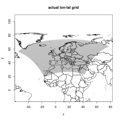
This is the actual geographic points, it shows a kind of fan of locations

#library(ncdf4)
library(ncdf)
library(raster)
projdir <- "~/projects/weather_european_eobs/eobs_temperature_tg_dataset"
outdir <- "data_provided"
outdir <- file.path(projdir, outdir)
#dir.create(outdir, recursive = T)
setwd(projdir)
dir()
# The URL below will get you the data, but the ECAD group do request you register your email address 
# they probably use this information to report some usage stats to their funders, so 
# Please do consider going to this webpage (http://www.ecad.eu/download/ensembles/ensembles.php)
# and register yourself.  Thanks!
webroot <- "http://www.ecad.eu/download/ensembles/data/Grid_0.22deg_rot"
# Create a list of netcdf files to download, we can loop over it
file_list <- c("tg_0.22deg_rot_1950-1964_v12.0.nc.gz","tg_0.22deg_rot_1965-1979_v12.0.nc.gz")

# only download if not already done
setwd(outdir)
for(i in 1:length(file_list))
    {
    dl <- file.path(webroot, file_list[i])
    dl
    infile <- basename(dl)
    exists  <- dir(pattern= infile)
    if(
      !exists("exists")
       )
    {
    download.file(dl, destfile = infile, mode = "wb")
    system(sprintf("gunzip %s", infile))
    }
    " (250MB)"
    }
setwd(projdir)

# now we can go through all days, I set this up as a loop over ncdf files then days, 
# but I'll probably try to set this up to directly use the netCDF aggregation functions available and avoid looping 
# for(j in 1:length(file_list))
  #{
    j = 1
    infile <- file.path(outdir, gsub(".gz", "", file_list[j]))
    nc <- open.ncdf(infile)
    #str(nc)
    print(nc)
    #?get.var.ncdf, following the example in the help file
    print(paste("The file has",nc$nvars,"variables"))
    var_i      <- nc$var[[4]]
    #var_i
    varsize <- var_i$varsize
    ndims   <- var_i$ndims
    nt      <- varsize[ndims]  # Remember timelike dim is always the LAST dimension!
    #nt 
    # we will set up to do a loop over days, I want to
    # a) read in the day grid
    # b) make a spatial points file with the appropriate projection
    # c) convert to geotiff and save to disk
    #for(i in 1:nt)
    #  {
        i = 1
       # Initialize start and count to read one timestep of the variable.
       start <- rep(1,ndims)   # begin with start=(1,1,1,...,1)
       start[ndims] <- i       # change to start=(1,1,1,...,i) to read timestep i
       count <- varsize        # begin w/count=(nx,ny,nz,...,nt), reads entire var
       count[ndims] <- 1       # change to count=(nx,ny,nz,...,1) to read 1 tstep
       data3 <- get.var.ncdf( nc, var_i, start=start, count=count )
        
       # Now read in the value of the timelike dimension
       timeval <- get.var.ncdf( nc, var_i$dim[[ndims]]$name, start=i, count=1 )
        
       print(paste("Data for variable",var_i$name,"at timestep",i,
               " (time value=",timeval,var_i$dim[[ndims]]$units,"):"))
       # [1] "Data for variable tg at timestep 1  (time value= 0 days since 1950-01-01 00:00 ):"      
       #print(data3)
       #image(data3)
       dat1 <- list()
       dat1$x <- get.var.ncdf(nc, varid="Actual_longitude")
       #dat1$x <- dat1$x[,1]       
       dat1$y <- get.var.ncdf(nc, varid="Actual_latitude")
       #dat1$y <- dat1$y[1,]              
       dat1$z <- get.var.ncdf(nc, var_i, start=start, count=count )
       str(dat1$z)
       #image(dat1$z)
       #map("world", xlim = c(xmin, xmax), ylim = c(ymin, ymax))
       #with(dat1, points(x, y, cex = .1, pch = 16))
       dat2 <- data.frame(
         x = as.vector(dat1$x),
         y = as.vector(dat1$y),
         z = as.vector(dat1$z)
         )
       #str(dat2)  
       #getwd()
       # I had the idea to save each day out to a file for looping over again and extracting spatially located data
       # say for a pixel, but I decided to try out the netCDF aggregation tools at a next step
       # save(dat2, file = sprintf("data_derived/eobs_tg_%s.RData",i))           
       #load(sprintf("eobs_tg_%s.RData",i))
       #This seemed like a good idea, but RData is more compressed
       # write.csv(dat2, sprintf("eobs_tg.csv",i), row.names = F, na = "")       
       #}
#}

# load the data for a specific day as example
dir("data_derived")
infile  <- "eobs_tg_1.RData"
load(file.path("data_derived/", infile))
ls()
# Now this is able to be mapped, but have make sure of the projection
library(maptools)
library(scales) 
library(RColorBrewer)
library(rgdal)
# the following code was adapted from

# Bedia, J. (2012). R practice using data from the ENSEMBLES
# Project. Retrieved from
# http://www.value-cost.eu/sites/default/files/VALUE_TS1_D02_RIntro.pdf

data(wrld_simpl)
# loads the world map dataset 
wrl  <- as(wrld_simpl,"SpatialLines") 
l1 <- list("sp.lines",wrl)
#x <- get.var.ncdf(nc, varid="Actual_longitude")
str(x)
x <- as.vector(x)
#y <- get.var.ncdf(nc, varid="Actual_latitude")
str(y)
y  <- as.vector(y)


coords <- cbind(x, y)
str(coords)
head(coords)
# so the actual lat lons are not regular grid in degrees
png("figures_and_tables/qc_actual_xy.png")
plot(coords, asp=1, cex=.4, col="grey", 
  pch="+", main=("actual lon-lat grid"))
lines(wrl)
dev.off()

This is the first graphic shown above, it shows a kind of fan of locations

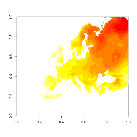
# so what does the rotated grid look like in its own universe?
str(dat1$z)
png("figures_and_tables/qc_rotated.png")
image(dat1$z)
dev.off()

This is how it looks on rotated grid

# so now add in the temperatures, use the wgs latlongs
t <- as.vector(dat1$z)
dat3 <- cbind.data.frame(coords, t)
summary(dat3)
coordinates(dat3) <- c(1,2)
#names(dat3@data)  <- c("z")
str(dat3)
summary(dat3@data)
color.palette <- rev(brewer.pal(11,"Spectral"))
getwd()
dir()
png("figures_and_tables/qc_tempmap_wgs.png")
spplot(dat3, scales=list(draw=TRUE), sp.layout=list(l1), 
       col.regions=alpha(color.palette,.2), cuts=10, 
       main="tg")
dev.off()

# write out the data to a shapefile
# we first have to make sure that the proj4 string is ok
str(dat3)
proj4string(dat3) <- "+proj=longlat +ellps=WGS84 +datum=WGS84 +no_defs +towgs84=0,0,0"
setwd(file.path(projdir, "data_derived"))
writeOGR(dat3, "out2.shp", "out2", "ESRI Shapefile")
setwd(projdir)

# to look at the rotated project do the following
# need to look at the website to get this info
# http://opendap.knmi.nl/knmi/thredds/dodsC/e-obs_0.22rotated/tg_0.22deg_rot_v12.0.nc.html
print(nc)
# it doesn't seem like there is this info in the ncdf file?
get.var.ncdf(nc, "projection")
rcm.lonlat.grid <- SpatialPoints(coords)
# now set this to wgs84
proj4string(rcm.lonlat.grid) <-"+proj=longlat +ellps=WGS84 +datum=WGS84 +no_defs +towgs84=0,0,0"

# this is the proj from website
# +proj=ob_tran +o_proj=longlat +lon_0=18 +o_lat_p=39.25 +a=6367470 +e=0
rcm.lambert.proj4 <- CRS("+proj=ob_tran +o_proj=longlat +lon_0=18 +o_lat_p=39.25 +a=6367470 +e=0")
# do the transform
spTransform(rcm.lonlat.grid, rcm.lambert.proj4) -> rcm.lambert.grid
summary(rcm.lambert.grid)

world.trans <- spTransform(wrl, rcm.lambert.proj4)

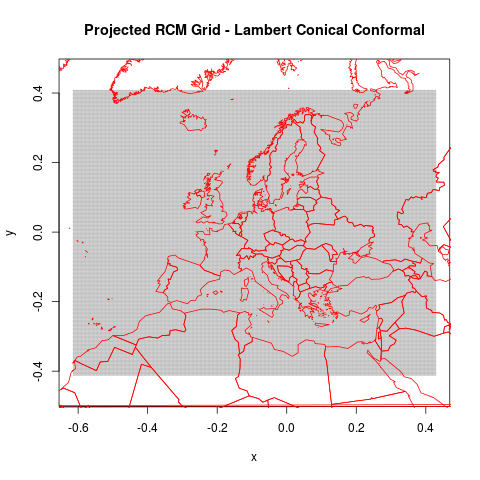
png("figures_and_tables/qc_rotated_grid_and_countries.png")
plot(rcm.lambert.grid@coords, cex=.2, pch=3, asp=1, col="grey", 
  main="Projected RCM Grid - Lambert Conical Conformal")
lines(world.trans, col="red")
dev.off()

This shows the rotated world countries

pr.df <- cbind.data.frame(coordinates(rcm.lambert.grid), dat3@data)
coordinates(pr.df) <- c(1,2) 
l1  <- list("sp.lines", world.trans)
color.palette <- colorRampPalette(c("yellow","cyan", "blue","purple"))

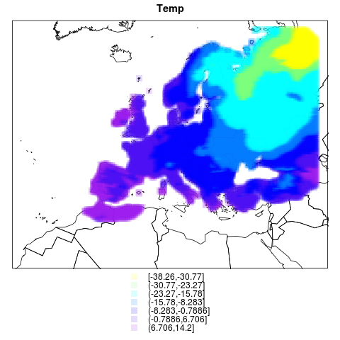
# This graph shows this with temp
png("figures_and_tables/qc_rotated_grid_and_countries2.png")
spplot(pr.df, sp.layout=list(l1), cuts=7, cex=1.5, 
  col.regions=alpha(color.palette(7),.15), pch=rep(15,7),
  main="Temp")
dev.off()
# not much point writing this to shapefile?
#proj4string(pr.df)  <- rcm.lambert.proj4
#str(pr.df)
#setwd(file.path(projdir, "data_derived"))
#dir()
# writeOGR(pr.df, "out.shp", "out", "ESRI Shapefile")

this one has temperatures too

acknowledgement and citations.

E-OBS temperature and precipitation:

We acknowledge the E-OBS dataset from the EU-FP6 project ENSEMBLES (http://ensembles-eu.metoffice.com) and the data providers in the ECA&D project (http://www.ecad.eu)

Haylock, M.R., N. Hofstra, A.M.G. Klein Tank, E.J. Klok, P.D. Jones, M. New. 2008: A European daily high-resolution gridded dataset of surface temperature and precipitation. J. Geophys. Res (Atmospheres), 113, D20119, doi:10.1029/2008JD10201”

According to Wikipedia https://en.wikipedia.org/wiki/Perfect_is_the_enemy_of_good this phrase was popularised by Voltaire, and Shakespeare via King Lear: “striving to better, oft we mar what’s well”

This phrase is a favourite of several people I respect and admire. On the other hand it has always vaguely troubled me. I think there may be two dimensions of this phrase that are worth pondering.

One: “the good” is a quality of the work

The first dimension is better expressed in King Lear, and on the wiki page where it is suggested the meaning is “that we might never complete a task if we have decided not to stop until it is perfect.” This is correct, however not an absolutely faithful interpretation of the phrase “striving to better”. To my mind this does not necessarily lead to the position “will not stop until perfect”. If one strives for perfection but admits that this is beyond the scope of one’s ambition then one will eventually stop when “it” is “good enough”, and that state will be better if one were striving for perfection than if one where aiming for “satisfactory”.

Two: “the good” is the impact the work may have on the world around us

The second dimension resonates more clearly with me and that is that “the good” is a public good, an impact that we feel would make the world a better place. To aim for a satisfactory action or intervention on the world around is would then be the goal, and we should try to achieve this as soon as possible, without delaying our work with minutia or trivia that might be that extra 1 percent that we would hope elevates our work further than satisfactory. One extra rung up the ladder toward perfection.

Stirzaker’s “simplicity cycle”

On page 175 of Stirzaker, R. (2010). Out of the scientists garden: A story of water and food. Canberra, Australia: CSIRO. I copied the image and show it below, but I have flipped it around so the axis are reversed from his original. This shows a couple of trajectories we can head along in terms of striving for enhancements, and the effect this has on how “good” the results are.

Seriousness aside

I used this image in my last project as a rallying call to the team to focus on both striving for the perfection while also balancing our aims to impact on the good. My colleagues pointed out that the flipped over version is easily turned into a stickman, a la XKCD!

• UPDATE to post http://ivanhanigan.github.com//2015/10/gis-issues-when-r-used-transforming-coordinate-systems
• Recall that RGDAL transforms and write out spatial data in GDA94 with a problem in that ArcGIS does not like the prj file and complains
• This seems an ok workaround

infile <- "western_sydney_passive_samplers_site_details.csv"
indir <- "data_derived"

outdir <- indir
outfile <- file.path(outdir, gsub(".csv",".shp",infile))

dat <- read.csv(file.path(indir, infile), as.is=T)
str(dat)
  
dat2 <- SpatialPointsDataFrame(data.frame(x=dat$long, y=dat$lat), dat,
                                proj4string=CRS(epsg$prj4[epsg$code %in% '4283'])
                                )

writeOGR(dat2, outfile,
         outdir, driver='ESRI Shapefile'
         )
# fix the prj file 
download.file("http://spatialreference.org/ref/epsg/4283/prj/",
              gsub(".shp", ".prj", outfile), mode = "wb"
              )

Some good reading and best-practice advice

• Driessen, V. (2010). A successful Git branching model. Nvie.Com. Retrieved January 28, 2016, from http://nvie.com/posts/a-successful-git-branching-model/

• Huff, K. D. (n.d.). A Software Release Checklist. Retrieved January 28, 2016, from http://bids.berkeley.edu/news/software-release-checklist

• Stanisic, L., Legrand, A., & Danjean, V. (2015). An Effective Git And Org-Mode Based Workflow For Reproducible Research. ACM SIGOPS Operating Systems …. Retrieved from http://dl.acm.org/citation.cfm?id=2723881

In my previous post I bemoaned the variability in definitions of reproducibility and replication.
The definition of reproducibility in particular concerns me as I finalise my thesis on ‘Reproducible Research Pipelines’. However I also have noticed a confusion of Repeatability and Replication that is worth noting. In various author’s definitions. In CASSEY, P., & BLACKBURN, T. M. (2006). Reproducibility and Repeatability in Ecology. BioScience, 56(12), 958. http://bioscience.oxfordjournals.org/content/56/12/958.full they agree with the definition of Peng 2011 that Reproducibility is to re-calculate the same result from the same data and they use Repeatability as a synonym for Peng’s Replication.

According to Cassey and Blackburn (2006), reproducibility is the case that:

from the information presented in the study, a third party could
replicate (sic) the reported results identically.

This definition distinguishes reproducibility from repeatability which is when

a third party must be able to perform a study using identical methodological protocols 
and analyze the resulting data in an identical manner

Which is what Peng terms ‘replicability’. This leads me to conclude that:

Cassey and Blackburn conflate Repeatability with Replicability.

However another author gives a very confused and overlapping view Ellison, A. (2010). Repeatability and Transparency in Ecological Research. Ecology. https://dash.harvard.edu/bitstream/handle/1/3123279/Ellison_Repeatability.pdf?sequence=2 Accessed 12 Jan 2016.

To add further confusion I have dug up the latest dictionary of epidemiology and find that whilst this agrees with Reproducibility and Replication, it treates Repeatability as a synonym of Reproducibility!

• Porta, Miquel S. Dictionary of Epidemiology (6th Edition). New York, NY, USA: Oxford University Press, USA, 2014. ProQuest ebrary. Web. 24 January 2016. Copyright © 2014. Oxford University Press, USA. All rights reserved.

Repeatability (Syn: reproducibility): The value below which the
absolute difference between two single test results may be expected to
lie with a probability of 95%, when the results are obtained by the
same method and equipment from identical test material in the same
setting by the same operator within short intervals of time. A test or
measurement is repeatable if the results are identical or closely
similar each time it is conducted. 1-3,5-9,91 See also measurement,
terminology of; reliability.

Replication: The execution of an observational or experimental study
more than once so as to confirm the findings, increase precision, and
obtain a closer estimation of sampling error. Exact replication should
be distinguished from consistency of results on replication. Exact
replication is often possible in the physical sciences, but in the
health, life, and social sciences consistency of results on
replication is often the best that can be
attained. 1,2,6,25,39,42,91,206-208,270,273,533 Consistency of results
on replication is perhaps the most important consideration in
judgements of CAUSALITY.

Reproducibility: see REPEATABILITY.

Whatever happens, never cite Drummond 2009!

It is unclear whether Drummond’s self-published conference paper was peer reviewed (or reviewed by the conference committee) but the following quote is unsupported assertion and should be ignored.

Reproducibility requires changes; replicability avoids them.

Drummond, C. (2009). Replicability is not Reproducibility: Nor is it Good Science. Proceedings of the Evaluation Methods for Machine Learning Workshop 26th International Conference for Machine Learning. Retrieved January 25, 2016, from http://cogprints.org/7691/7/icmlws09.pdf

Indeed in 2012 Drummond (in another self-published, working paper without evidence of peer review) did a backflip and said:

Reproducibility requires that the experiment originally carried out be duplicated 
as far as is reasonably possible. The aim is to minimize the difference from 
the first experiment including its flaws, to produce
independent verification of the result as reported

Drummond, C. (2012). Reproducible research: A dissenting opinion. Unpublished draft. Retrieved October 9, 2015, from http://cogprints.org/8675/