Welcome to my Open Notebook

This is an Open Notebook with Selected Content - Delayed. All content is licenced with CC-BY. Find out more Here.

ONS-SCD.png

Timeseries with Spatial Lag

adjacency example

adjacency example


1 Introduction

I've got a timeseries model I am fitting to a city dataset with about 45 zones. The data are daily, stratified by Zone, Age and Sex. Following on from learning about spatiallly correlated errors I want to see if the Standard Error on the estimated \(\beta_{1}\) from the timeseries model is affected.

I think the simplest option is to use the spatial lag model, which can be fitted with just adding a term that is the average of the set of each Zone's neighbours outcome level on each day. For this I need to find the list of each region's neighbours. Then I'll use this to assign each zone/day/age group their neighbours values and then collapse that to get their daily means.

2 Load some test data

# we have access to a classic dataset for studying spatial dependence
# in the spdep package
if(!require(spdep))    install.packages(spdep); require(spdep)     
if(!require(rgdal))    install.packages(rgdal); require(rgdal) 
if(!require(maptools)) install.packages(maptools); require(maptools) 
if(!require(maps))     install.packages(maps); require(maps) 
fn <- system.file("etc/shapes/eire.shp", package="spdep")[1]
prj <- CRS("+proj=utm +zone=30 +units=km")
eire <- readShapeSpatial(fn, ID="names", proj4string=prj)
str(eire)
# reproject into a better coordinate system
eire <- spTransform(eire, CRS("+proj=longlat +datum=WGS84"))
# check out the attributes
head(eire@data)

AtownspalesizeROADACCOWNCONSPOPCHGRETSALEINCOMEnames
34.20.121108736648.69729627185Carlow
29.680.01021335000156944529459Cavan
26.540.01053543211978346012435Clare
23.920.030147641189902840265901Cork
27.910.03098975002775747817626Donegal
32.790.6111810530789.414289424164631Dublin

3 spdep calculates neighbours

nb <- poly2nb(eire)
str(nb)
#List of 26
nb[[1]]
#[1]  9 10 11 25 26
# So this returns the set of index values for each area's neighbours
# I'd prefer to read their names
eire[['names']][1]
# > [1] Carlow
# so therefore the neighbours of area 1 "Carlow" are in the first
# element of the list
eire[['names']][nb[[1]]]
# > [1] Kildare  Kilkenny Laoghis  Wexford  Wicklow

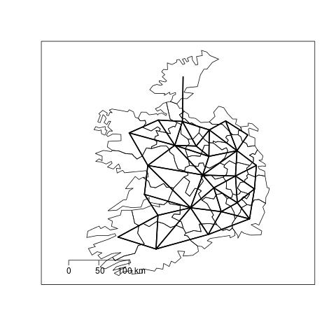
4 plot these

################################################################
# name:plot these
png("images/Fig1.png")
plot(eire)
plot(nb, coordinates(eire), add=TRUE, pch=".", lwd=2)
map.scale(ratio = F)
box()
dev.off()
images/Fig1.png

5 function to return adjacency list as a dataframe

I THINK I actually want this as a dataframe so I can merge it with the master table of outcome data.

################################################################
# name:adjacency_df
adjacency_df <- function(NB, shp, zone_id)
  {
    adjacencydf <- as.data.frame(matrix(NA, nrow = 0, ncol = 2))
    for(i in 1:length(NB))
    {
      if(length(shp[[zone_id]][NB[[i]]]) == 0) next
      adjacencydf <- rbind(
                           adjacencydf,
                           cbind(
                                 as.character(shp[[zone_id]][i]),
                                 as.character(shp[[zone_id]][NB[[i]]])
                                 )
                           )
    }
    return(adjacencydf)
  }

6 test-adjacency df

################################################################
# name:adjacency_df
adj <- adjacency_df(NB = nb, shp = eire, zone_id = 'names')
adj  
CarlowKildare
CarlowKilkenny
CarlowLaoghis
CarlowWexford
CarlowWicklow
CavanLeitrim
CavanLongford
CavanMeath
CavanMonaghan
CavanWestmeath
ClareGalway
ClareLimerick
ClareTipperary
CorkKerry
CorkLimerick
CorkTipperary
CorkWaterford
DonegalLeitrim
DublinKildare
DublinMeath
DublinWicklow
GalwayClare
GalwayMayo
GalwayOffaly
GalwayRoscommon
GalwayTipperary
KerryCork
KerryLimerick
KildareCarlow
KildareDublin
KildareLaoghis
KildareMeath
KildareOffaly
KildareWicklow
KilkennyCarlow
KilkennyLaoghis
KilkennyTipperary
KilkennyWaterford
KilkennyWexford
LaoghisCarlow
LaoghisKildare
LaoghisKilkenny
LaoghisOffaly
LaoghisTipperary
LeitrimCavan
LeitrimDonegal
LeitrimLongford
LeitrimRoscommon
LeitrimSligo
LimerickClare
LimerickCork
LimerickKerry
LimerickTipperary
LongfordCavan
LongfordLeitrim
LongfordRoscommon
LongfordWestmeath
LouthMeath
LouthMonaghan
MayoGalway
MayoRoscommon
MayoSligo
MeathCavan
MeathDublin
MeathKildare
MeathLouth
MeathMonaghan
MeathOffaly
MeathWestmeath
MonaghanCavan
MonaghanLouth
MonaghanMeath
OffalyGalway
OffalyKildare
OffalyLaoghis
OffalyMeath
OffalyRoscommon
OffalyTipperary
OffalyWestmeath
RoscommonGalway
RoscommonLeitrim
RoscommonLongford
RoscommonMayo
RoscommonOffaly
RoscommonSligo
RoscommonWestmeath
SligoLeitrim
SligoMayo
SligoRoscommon
TipperaryClare
TipperaryCork
TipperaryGalway
TipperaryKilkenny
TipperaryLaoghis
TipperaryLimerick
TipperaryOffaly
TipperaryWaterford
WaterfordCork
WaterfordKilkenny
WaterfordTipperary
WaterfordWexford
WestmeathCavan
WestmeathLongford
WestmeathMeath
WestmeathOffaly
WestmeathRoscommon
WexfordCarlow
WexfordKilkenny
WexfordWaterford
WexfordWicklow
WicklowCarlow
WicklowDublin
WicklowKildare
WicklowWexford

</html>

Posted in  spatial dependence


Reflections on Spatial Regression Class with Prof Bob Haining

Reflections on a class with Prof Bob Haining

1 Introduction

I recently attended a class on spatial regression with Prof Bob Haining. He described the issue of spatially correlated errors and the problems this poses in spatial regression.

The key issue is that spatial data often violates the assumption in regression models that the errors are independent.

A simple regression model applied to spatial data based on ZONES:

\(Y_{i} = \beta_{0} + ZONE_{i} + \beta_{1} X_{1i} + e_{i}\)

But with spatial data it is likely that the errors are spatially correlated. This is likely to mean the point estimate of beta 1 is OK but the Standard Error is wrong.

This might be due to the scale of the study units, which may not capture the variation of exposure and outcome adequately. Or there might be unmeasured explanatory variables that have not been accounted for.

I am mostly concerned with EXPLANATORY modelling in which a particular exposure of interest is to be assessed. Examples include a weather variable (temperature), an air pollutant (PM10) or some measure of socio-economic deprivation in an area (SEIFA scores in Australian census data). In these models I tend to include a number of 'nuisance' parameters to control for confounding; or interaction terms to account for effect modification. In this type of model the performance of the model over-all is not that important, I just want to control for the most important confounders so that my estimate of the exposure of interest is as rigorous as possible.

Therefore the problem that spatially correlated errors pose for these models is slightly different to that which affects models aimed at PREDICTION: I am not concerned so much with the model's fit to the data, rather the confidence around the point-estimate of the parameter for the exposure of interest.

Simplistically I took away the following messages:

2 The Spatial Error Model

So we could model allowing for correlated errors:

\(Y_{i} = \beta_{0} + ZONE_{i} + \beta_{1} X_{1i} + \eta_{i}\)

Where:

\(\eta_{i}\) = Spatially autocorrelated errors.

3 The Spatial Lag Model

Or we could include a term for the neighbours, thus absorbing the correlated errors:

\(Y_{i} = \beta_{0} + ZONE_{i} + \beta_{1} X_{1i} + \rho(Neighbours Y_{ij}) + e_{i}\)

Where:

\(\rho_(Neighbours Y_{ij})\) = is an additional explanatory variable which is the value of the dependent variable in neighbouring areas.

4 Spatially Lagged Independent Variable(s)

This is almost a variation of the spatial lag model, except that we include a term for the exposure variable in the neighbours, and therefore 'smooth' the effect of the exposure from what was observed in any area to make it relevant to it's neighbours as well:

\(Y_{i} = \beta_{0} + ZONE_{i} + \beta_{1} X_{1i} + \beta_{2L} X_{2ij} + e_{i}\)

Where:

\(\beta_{2L} X_{2ij}\) = is the independent variable X2 that is spatially lagged.

5 Discussion

5.1 How to decide which model to fit?

So the burning question is how to choose between the various spatial models? Prof Haining had some suggestions, but he noted that sometimes two could be equally appropriate. He suggested that the spatial lag model makes the strong assumption that there is a relationship between the outcome in a neighbouring area with the index zone. This suggests some kind of contagion or dispersion effect. He was not keen to fit this model in circumstances where the causal mechanism did not support such a relationship, suggesting the spatially weighted error model was more suited, but that "in practice they often give the same result".

In my situation where I am not concerned with the actual autocorrelation but with tightening up the standard error on my exposure of interest, I think I might plead forgiveness and try fitting the spatial lag model as it seems easier.

6 Conclusion

Stay tuned.

</html>

Posted in  spatial dependence


software-ism

I am a huge fan of the R language for statistics and graphics.

I sometimes hear people say they don’t like R but then admit that they have never tried to use it, or if they have it was close to ten years ago (and a lot has changed).

In recent discussions at work I got the impression some people have got a bit predjudiced against R and other software that they don’t actually use, primarily because of the added difficulty of software that requires a bit of programming.

I think that multi-disciplinary work will inevitably mean we find a mix of software in use, and they’ll all have strengths and weaknesses. A major strength of R is that one can weave together a report that includes the data, code, graphs and interpretations for an analysis, rather than copy-and-pasting these elements together as is required with other software toolboxes.

For example a simple analysis in Rstudio using the ‘R Markdown document’ is below.

You can load and explore data in the document by placing ‘Code Chunks’ in the document, then when you click the Knit HTML button a web page will be generated that includes both content as well as the output of any embedded R code chunks within the document. You can embed an R code chunk like this:


summary(cars) --- 

| speed | dist | |————–|—————- | Min. : 4.0 | Min. : 2.00
| 1st Qu.:12.0 | 1st Qu.: 26.00
| Median :15.0 | Median : 36.00
| Mean :15.4 | Mean : 42.98
| 3rd Qu.:19.0 | 3rd Qu.: 56.00
| Max. :25.0 | Max. :120.00

You can also embed plots, for example:


plot(cars)

plot of chunk unnamed-chunk-2

I hope we can work toward a kind of ‘tower of babel’.

Posted in  research methods


The Ecological Fallacy is Itself a Fallacy

The Ecological Fallacy

The term ‘Ecological fallacy’ is used in Epidemiology and some other disciplines (such as Sociology) to refer to improperly inferring a causal association (or lack of association) at an individual-level based on a group-level relationship. This use of the word ecological is at odds with the alternative use of the word in the discipline of Ecology. Ecological methods from Ecology are inherently multi-scaled and address precisely the issue of this cross-scale inferential fallacy.

I argue that a broader understanding of ecological methods by non-Ecologists would be a start towards better understanding between the disciplines. The inclusion of real ecological methods in the other disciplines will also assist research to better understand the causes and effects of climate and climate change which are important gaps in knowledge needed to enable mitigation and adaptation of our society to future climate change.

Sociology

To clear up this confusion it is necessary to go back to the source of the use of the term ‘ecological’ by the urban sociologist Amos Hawley who used the term ‘human ecology’ in the 1950s to build on the theoretical traditions of Robert Parke and E. W. Burgess at the University of Chicago in the 1920s on the structure and development of cities. His influence in the Social Sciences led directly to the development a tradition of social human ecology, one largely without a bio-physical environment. The usage of ‘ecological’ to mean multivariate studies of complex systems stems from the sociological tradition.

Ecology

The term ‘ecology’ used in the Ecology discipline dates back to the 1870s, coined by German zoologist Ernst Haeckel (1834-1919) as Oekologie from Greek ‘oikos’ for house, dwelling place, habitation and ‘logia’ study of, then at the turn of the century the term became spelt ‘oecology’, which grew into ‘ecology’ in the early part of the 1900s.

Epidemiology

In epidemiology the term ‘ecological study’ is used to refer to studies where observations are taken at the level of a group (such as a country, school, or hospital) rather than at the individual (such as patient) level. It is well known though that when risk factors and outcomes are measured at an aggregate level, the relationship between the group-level variables may be different than the relationship between variables measured at the individual level. An often cited example used to illustrate the issue involved a 19th century study which found higher suicide rates within Prussian provinces that had higher proportions of Protestant residents. The conclusion that Protestant individuals (rather than Catholic individuals) were more likely to commit suicide cannot be inferred based on the observed association among the provinces. One possible scenario is that Catholic residents within the largely Protestant provinces had the high suicide rates, resulting in a positive association between percent Protestant and suicide rate 8. Extrapolation of aggregate results to individuals is a mistake in logic 9 which can lead to a potentially misleading conclusion 10.

Because of this limitation ‘ecologic studies’ are often scorned in epidemiology as inferior and only useful for exploratory or hypothesis-generating studies rather than as confirmatory. I argue to the contrary that there is the potential for a revolution in our ability to understand causal influences operating at multiple scales of space and time if we were to conduct truly ‘ecological studies’.

Quantitative Geography

There is also a closely related concept that should be noted. That of the Modifiable Areal Unit Problem (MAUP) as discussed in quantitative geography. There is a large amount of geographical literature on the MAUP. In this problem domain areal units (also called zones, regions, areas or polygons) inherently pose three problems to a researcher attempting to infer causal associations: scale, zonal and temporal:

  • Scale; this issues is evident in the example above where phenomena investigated using data viewed at one scale may appear quite different (even opposite) using data aggregated at a different scale.
  • Zonal; the zonal problem appears where phenomena investigated using data viewed using two sets of differing areas at a single scale can differ.
  • Temporal; a third problem arises when analyzing data on modifiable areas when people keep modifying them by redrawing the boundaries over time.

In Conclusion

The term ‘Ecological Fallacy’ is itself a fallacy and non-Ecologists should be made aware of the existence of alternative ecologic methods from Ecology. This would be a start towards better understanding between the disciplines and enhance our abilities to mitigate and adapt to climate change.

Posted in  research methods


Centennial Scale Rainfall in Southeastern Australia

Droughts are extreme rainfall events on centennial scale

In the Hutchinson Drought Index project we used the longest period of rainfall data available because the drought index is based on the ranking of each six-month average of the distribution in the entire record of observations. A period as long as this is required to calculate extreme rainfall deficits. The original Hutchinson paper used a period 1920-1988 due to availability. Another consideration is the longer term characteristics of the rainfall epoch you are considering.

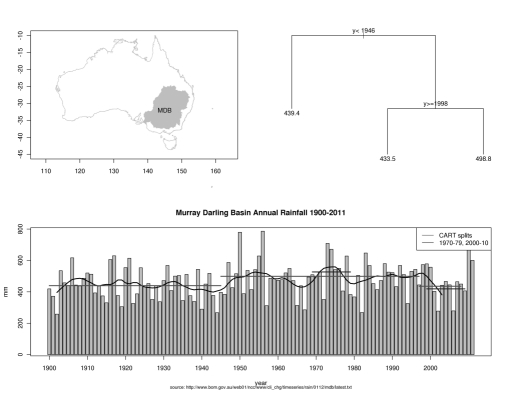
For example, in recent decades in Southeastern Australia annual total rainfal does not represent the longer term context very well. Shown in the image below is the result of an exploratory data analysis using rainfall data from the Murray Darling Basin (the ‘bread basket’ of Australian agriculture). I use the Classification And Regression Tree tool in the ‘rpart’ package to determine the optimal groupings. I’ve dropped the last two years of the sequence because when I first ran this analysis two years ago I got the result shown, but thankfully the last two years have given us very good rainfalls. This shows the difference between short-term and long-term rainfall patterns.

Regardless of this data ‘massaging’, in the analysis presented the annual trend over the first half of the twentieth century was lower than the recent fifty years, by about 60 millimeters on average. The 1930-1946 period was particularly dry, as has been the 1998-2008 period.

plot of seaust rainfall

Posted in  extreme weather events