- Thinking about this again, it should be possible to use the pixel values to get the drought areas based on the colour.
![]()
This is an Open Notebook with Selected Content - Delayed. All content is licenced with CC-BY. Find out more Here.

![]()
Posted in drought awap grids data operation
05 Sep 2016
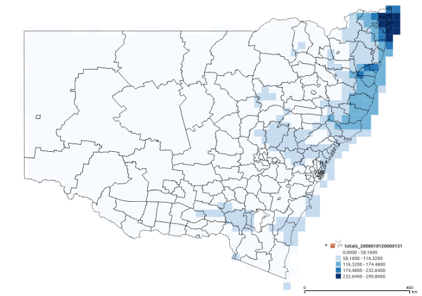
Drought Declarations are made by government in Australia to determine when and where a drought is occuring. The Declarations are linked to agricultural and social support policies. We are working on a climatic drought index that should correlate with these Drought Declarations. The New South Wales Government has provided us with spatial data from 1986 but they also have a graphical visualisation available for earlier times, especially noteworthy is the extreme 1982-1983 drought. This post is a document of the process I will try to derive spatial data from the image.
Download the drought maps. The current maps are at: http://www.dpi.nsw.gov.au/content/agriculture/emergency/drought/planning-archive/climate/advance-retreat
But there is a higher resolution map archived at: http://pandora.nla.gov.au/pan/120345/20120529-0000/advance-retreat-drought-map-april-2011.pdf
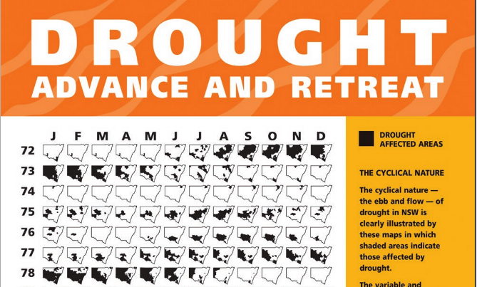
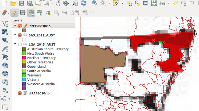

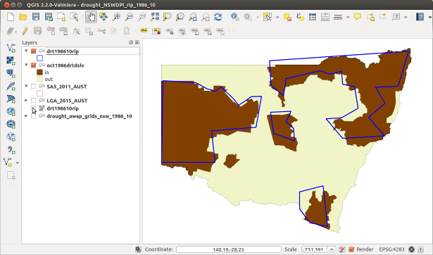
The process produces data that is very prone to imprecision. We may be able to use some extra data from before 1986 though.
Posted in drought awap grids data operation
30 Aug 2016
Posted in drought awap grids
27 Aug 2016
### Load the package or install if not present
if (!require("RColorBrewer")) {
install.packages("RColorBrewer")
library(RColorBrewer)
}
## Loading required package: RColorBrewerpar(mfrow = c(3,3))
for(col_i in c('YlGn','RdPu', 'PuRd', 'BrBG', 'RdBu', 'RdYlBu', 'Set3', 'Set1')){
display.brewer.pal(n = 5, name = col_i)
}
for(col_i in c('YlGn','RdPu', 'PuRd', 'BrBG', 'RdBu', 'RdYlBu', 'Set3', 'Set1')){
  print(col_i)
  print(brewer.pal(n = 5, name = col_i))
}
## [1] "YlGn"
## [1] "#FFFFCC" "#C2E699" "#78C679" "#31A354" "#006837"
## [1] "RdPu"
## [1] "#FEEBE2" "#FBB4B9" "#F768A1" "#C51B8A" "#7A0177"
## [1] "PuRd"
## [1] "#F1EEF6" "#D7B5D8" "#DF65B0" "#DD1C77" "#980043"
## [1] "BrBG"
## [1] "#A6611A" "#DFC27D" "#F5F5F5" "#80CDC1" "#018571"
## [1] "RdBu"
## [1] "#CA0020" "#F4A582" "#F7F7F7" "#92C5DE" "#0571B0"
## [1] "RdYlBu"
## [1] "#D7191C" "#FDAE61" "#FFFFBF" "#ABD9E9" "#2C7BB6"
## [1] "Set3"
## [1] "#8DD3C7" "#FFFFB3" "#BEBADA" "#FB8072" "#80B1D3"
## [1] "Set1"
## [1] "#E41A1C" "#377EB8" "#4DAF4A" "#984EA3" "#FF7F00"# or for more levels
brewer.pal(n = 10, name = "RdYlBu")## [1] "#A50026" "#D73027" "#F46D43" "#FDAE61" "#FEE090" "#E0F3F8" "#ABD9E9"
## [8] "#74ADD1" "#4575B4" "#313695"The leading # is just there by convention. Parse the hexadecimal string like so: #rrggbb, where rr, gg, and bb refer to color intensity in the red, green, and blue channels, respectively. Each is specified as a two-digit base 16 number, which is the meaning of "hexadecimal" (or "hex" for short). Here's a table relating base 16 numbers to the beloved base 10 system.### Show all the colour schemes available
par(cex = .6)
display.brewer.all()
### Set the display a 2 by 2 grid
par(mfrow=c(2,2))


### Generate random data matrix
rand.data <- replicate(8,rnorm(100,100,sd=1.5))

### Draw a box plot, with each box coloured by the 'Set3' palette
boxplot(rand.data,col=brewer.pal(8,"Set3"))

### Draw plot of counts coloured by the 'Set3' pallatte
br.range <- seq(min(rand.data),max(rand.data),length.out=10)
results <- sapply(1:ncol(rand.data),function(x) hist(rand.data[,x],plot=F,br=br.range)$counts)
plot(x=br.range,ylim=range(results),type="n",ylab="Counts")
cols <- brewer.pal(8,"Set3")
lapply(1:ncol(results),function(x) lines(results[,x],col=cols[x],lwd=3))

### Draw a bar chart
table.data <- table(round(rand.data))
cols <- colorRampPalette(brewer.pal(8,"Dark2"))(length(table.data))
barplot(table.data,col=cols)
Posted in exploratory data analysis
03 Aug 2016
'name:poa06-area-lambert'
setwd("~/projects/POA_centroids/POA2006_centroids")
library(swishdbtools)
ch <- connect2postgres2("delphe")

fout_geo=dbGetQuery(ch,
'select poa_2006,
  st_area(st_transform(the_geom, 3112))/1000000 as Geoscience_Australia_Lambert_area_km2,
st_x(st_centroid(st_transform(the_geom,3112))) as geocentx,
st_y(st_centroid(st_transform(the_geom,3112))) as geocenty
from abs_poa.auspoa06')
str(fout_geo)
sum(fout_geo$geoscience_australia_lambert_area_km2)
write.table(fout_geo,'data_derived/auspoa06_geocentroids_lambert_20160624.csv',
            row.names=F, sep=',')

plot(fout_geo[,3:4])
head(fout_geo)
nrow(fout_geo)
2507
Posted in spatial
24 Jun 2016


