• I have been using John Myles Whites ProjectTemplate R package for ages
• I really like the ease with which I can get up and running a new project
• and the ease with which I can pick up an old project and start adding new work

Quote from John’s first post

My inspiration for this approach comes from the rails command from
Ruby on Rails, which initializes a new Rails project with the proper
skeletal structure automatically. Also taken from Rails is
ProjectTemplate’s approach of preferring convention over
configuration: the automatic data and library loading as well as the
automatic testing work out of the box because assumptions are made
about the directory structure and naming conventions that will be used

http://www.johnmyleswhite.com/notebook/2010/08/26/projecttemplate/

• I dont know anything about RoR but this philosophy works really well for my R programming too

R Code

if(!require(ProjectTemplate)) install.packages(ProjectTemplate); require(ProjectTemplate)
setwd("~/projects")
create.project("my-project")
setwd('my-project')
dir()
##  [1] "cache"       "config"      "data"        "diagnostics" "doc"        
##  [6] "graphs"      "lib"         "logs"        "munge"       "profiling"  
## [11] "README"      "reports"     "src"         "tests"       "TODO"   
##### these are very sensible default directories to create a modular
##### analysis workflow.  See the project homepage for descriptions
 
# now all you need to do whenever you start a new day 
load.project()
# and your workspace will be recreated and any new data automagically analysed in
# the manner you want

Project Administration

• I;ve found that these directories do not work so well for the administration of my projects and so I put together a different set of automatic defaults
• Ive based it on the University of Manitoba Centre for Health Policy- along with some other sources I can recall

  The full set

  # A.Background
  # B.Proposals # C.Approvals # D.Budget
  # E.Datasets
  # F.Analysis
  # G.Literature
  # H.Communication
  # I.Correspondance
  # J.Meetings
  # K.Completion
  # ContactDetails.txt
  # README.md # TODO.txt

R Code: my subset

AdminTemplate <- function(rootdir = getwd()){
  setwd(rootdir)
  dir.create(file.path(rootdir,'01_planning'))
  dir.create(file.path(rootdir,'01_planning','proposal'))
  dir.create(file.path(rootdir,'01_planning','scheduling'))
  dir.create(file.path(rootdir,'02_budget'))
  dir.create(file.path(rootdir,'03_communication'))
  dir.create(file.path(rootdir,'04_reporting_and_meetings'))
  file.create(file.path(rootdir,'contact_details.txt'))
  file.create(file.path(rootdir,'README.md'))
  }

Conclusion

• hopefully by formalising some of these into my workflow I will find my projects easier to navigate through
• and pick up or put down as needed

• Studies of extreme weather events such as drought require long term climate data
• these are available at continental scale derived from
• observations from a network of weather stations that are interpolated to a surface
• I have been working on techniques with R and online resources (the Australian Water Availabilty Project AWAP) to make working with these long term climatology datasets easier.
• The package is in development at https://github.com/swish-climate-impact-assessment/awaptools

Case Study

• aim is need to look at seasonal rainfall means.
• first thing is to download the data (I’m also working on a Rstudio server to host these data, as a Virtual Lab).
• data = multiple years of monthly rainfall data in a raster grid format.
• aim = combine rainfall in a seasonal basis in one grid
• (i.e. M-J-J-A-S-O 1900, 1901 etc.) calculate mean of each cell.
• assumption1 = filenames have year, month embedded so they will be sorted in order when listed
• assumption2 = all months are available, from 1:12 for all years in
• study period
• notes:
• this requires the files are listed in the right order by name, and all months are present. might be better to use grep on the file name and strsplit/substr to extract the month identifier more precisely?

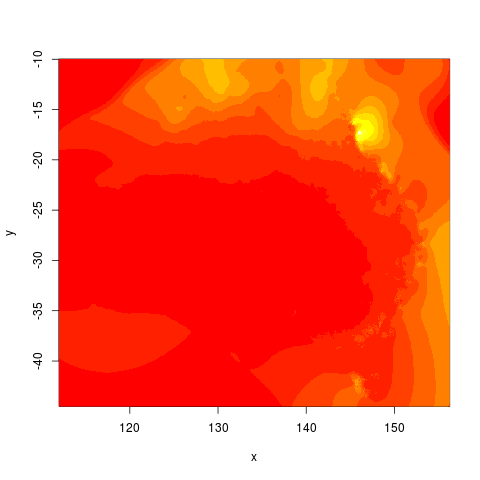
Results

I’m looking for collaboration on this!

• I’ve been in contact with:
• https://github.com/RationShop/rain_r/wiki/The-Rain-Project
• I apologise to windoze users but feel a bit like this guy when recomending how to install:

quote:

probably the easiest way to do this is to use
Hadley's devtools package.  Assuming you have devtools and my package's
dependencies.  If you're using Linux or the BSD's, this should just
work.  Welcome to the good life, player.  I think this will work out
of the box on a Mac.  I have no idea if this will work on Windows; how
you strange people get anything done amazes me.  At the least,
Im guessing you have to install Rtools first.  
You could also just source all the R scripts like 
some kind of barbarian

R Code:

# depends
require(swishdbtools)
if(!require(raster)) install.packages("raster", dependencies = T); require(raster)
if(!require(rgdal)) install.packages("rgdal", dependencies = T); require(rgdal)

# on linux can install direct, on windoze you configure Rtools
require(devtools)
install_github("awaptools", "swish-climate-impact-assessment")
require(awaptools)

homedir <- "~/data/AWAP_GRIDS/data"
outdir <- "~/data/AWAP_GRIDS/data-seasonal-vignette"
 
# first make sure there are no left over files from previous runs
#oldfiles <- list.files(pattern = '.tif', full.names=T) 
#for(oldfile in oldfiles)
#{
#  print(oldfile)
#  file.remove(oldfile)
#}
################################################
setwd(homedir)
 
# local customisations
workdir  <- homedir
setwd(workdir)
# don't change this
years <- c(1900:2014)
lengthYears <- length(years)
# change this
startdate <- "2013-01-01"
enddate <- "2014-01-31"
# do
load_monthly(start_date = startdate, end_date = enddate)
 
# do
filelist <- dir(pattern = "grid.Z$")
for(fname in filelist)
{
  #fname <- filelist[1]
  unzip_monthly(fname, aggregation_factor = 1)
  fin <- gsub(".grid.Z", ".grid", fname)
  fout <- gsub(".grid.Z", ".tif", fname)
  r <- raster(fin)
  writeRaster(r, fout, format="GTiff",  overwrite = TRUE)
  file.remove(fin)
}
 
cfiles <- list.files(pattern = '.tif', full.names=T) 
# loop thru
# NEED TO SET THE FILESOFSEASEON_I counter EACH TIME YOU start
 
 
for(season in c("hot", "cool"))
{
  # season <- "hot" # for labelling
  if(season == "cool")
  {
    filesOfSeason_i <- c(5,6,7,8,9,10)  
    endat <- lengthYears
  } else {
    filesOfSeason_i <- c(11,12,13,14,15,16) 
    endat <- lengthYears - 1
  }
  
  for (year in 1:endat){ 
    ## setup for checking month 
    # year  <- 1 #endat
    
    
    ## checking
    print(cat("####################\n\n"))
    print(cfiles[filesOfSeason_i])
    
    b <- brick(stack(cfiles[filesOfSeason_i])) 
    ## calculate mean 
    m <- mean(b) 
    ## checking 
    # image(m) 
    writeRaster(m, file.path(outdir,sprintf("season_%s_%s.tif", season, year)), drivername="GTiff")
    filesOfSeason_i <- filesOfSeason_i + 12
  } 
}
 
##### now we will overall average
setwd(outdir)
for(season in c("cool", "hot"))
{
  cfiles <- list.files(pattern = season, full.names=T)   
  print(cfiles)
  b <- brick(stack(cfiles)) 
  ## calculate mean 
  m <- mean(b) 
  ## checking 
  # image(m) 
  writeRaster(m, file.path(outdir,sprintf("season_%s.tif", season)), drivername="GTiff")
}
 
# qc
cool <- raster("season_cool.tif")
hot <- raster("season_hot.tif")
par(mfrow = c(2,1))
image(cool)
image(hot)
 
# just summer rainfall
png("season_hot.png")
image(hot)
dev.off()

Toward a standard and unambiguous format for sharing Year-Month data

• I am working in a new job where we are recieving data from a lot of different groups
• we aim to review these datasets and then publish them for a wide audience of potential users
• therefore usability and interoperability is a key concern
• we recieved some data with Month and Year as Apr.12
• I know this is easy to convert to a date/time class with in R but wondered what a better format would be to recommend for our datasets to use to maximise utility downstream (especially for non R users)
• Apr.12 is assumed to be text in excel so need something else
• Apr-12 is assumed to be the twelfth of April this year (ie 12/4/2014)

In R the solution might be to use the zoo package

require(zoo)
as.yearmon("Apr.12", "%b.%y")
# [1] "Apr 2012"

# other options abound
as.yearmon("apr12", "%b%y")

# the default is YYYY-MM or similar
as.yearmon("2012-04")
as.yearmon("2012-4")

• So I went looking at how Excel and Access deal with this
• found that the best appeard to be MMM-YYYY in terms of how these software assume the data should look

R Code:

as.yearmon("Apr-2012", "%b-%Y")

# but will need to specify format because otherwise fails
as.yearmon("Apr-2012")
# NA

Conclusion

• I recommend the MMM-YYYY option
• it is pretty good that in Excel it is assumed 1/04/2012
• and if MS access is set to date/time and format = mmm-yyyy is ok for data entry (but not importing)
• to import this use a shorttext type, then post-import, change to date/time with mmm-yyyy (the . failed)

Background

• “Blogging like a Hacker” has become a paradigm for programmers who want to link their code to their blogs.
• I’ve followed this paradigm for a while to support my scientific projects, enhancing their transparency and reproducibility.
• I’ve started a new project where I need to also manage project management and planning (following Tomas Aragon’s tutorial)
• I propose that the same methods I use in scientific programming and blogging like a hacker can be used in “Gantting like a Hacker”

• The title for this post is also influenced by the poste over at [Geek

  Manager](http://blog.geekmanager.co.uk/2007/05/02/using-the-best-plan-format/).

• That post says taht “Premature Gannting” is the act of making a “huge Gantt chart (often in MS Project).”
• Gannting like a Hacker is doing this in a scripted environment, without relying on closed-source proprietry software such as the Windoze options.
• The community of bloggers (mostly geeks) who are following a style of blogging that originated with the invention of Jekyll, unveiled in this post by Tom Preston-Werner; GitHub’s co-founder (aka mojombo).
• This experiment uses Taskjuggler and Emacs Orgmode

Materials and Methods

• Use Ubuntu 12.04 Long Term Support (LTS)
• with Ruby

Code:install task juggler

gem install taskjuggler

Gantt charts with Emacs Orgmode

• I’m using an Emacs tool to use TaskJuggler to handle the task scheduling and creation of Gantt chart suitable for a Pointy-haired Boss.
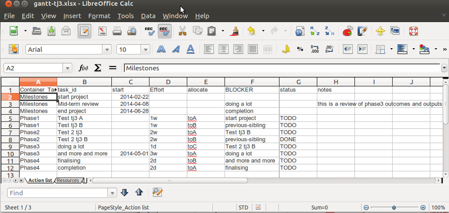
• I hated using the Orgmode script to compile the parts of the Gantt chart so I wrote this R script to convert a spreadsheet into an Orgmode script
• the spreadsheet is organised in a fairly simple way shown below.

Results

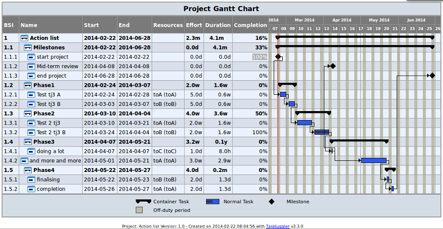
• and executing my script will convert this into a Emacs orgmode file that will export to a taskjuggler file (use C-c C-e j) and viola!

Conclusions

• This simplifies the Orgmode taskjuggler creation
• A drawback is that it has to go through the Emacs export function.

Reproducibility

• A subset of the data and code used for this blog post is available at https://github.com/ivanhanigan/aggregation-of-slas-or-sa2s
• Some parts of the data I used are not available due to shared Intellectual Property
• The spatial data and SEIFA Socioeconomic index data are publicly available from the Australian Bureau of Statistics
• The New Groups categories were generously contributed by John Glover of the Public Health Information Development Unit, The University of Adelaide.

Introduction

The Aim is to aggregate Statistical Local Areas (SLAs, recently relabelled SA2) Australian Standard Geographical Classification (ASGC, recently relabelled ASGS) to achieve a greater level of privacy protection. The rules to achieve a geography amenable to statistical comparisons are:

• similar populations (around 20,000 to 30,000)
• homogenous Index of Relative Socioeconomic Disadvantage
• nested within the next level up in the ASGC/ASGS
• so that SSD (recently relabelled SA3) are not split.
• the SA2s can be aggregated through a process of assigning alike areas to groups, and reviewing/adjusting these assignments
• This document contains some suggestions for adjusting groupings to better reflect differences in the level of disadvantage, while still adhering to the rules outlined.

Results

Data Prep

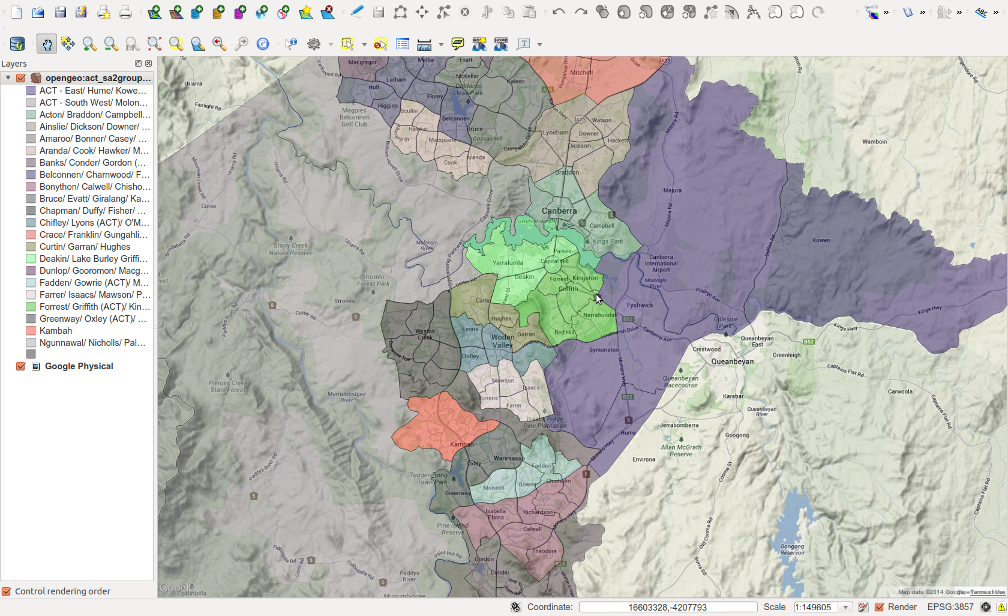
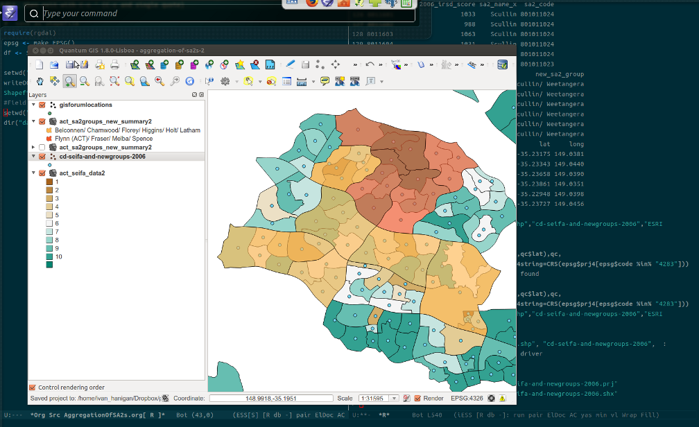
• The data were prepared as spatial files

Assess proposed split in Belconnen

• the proposed split in belconnen looks good
• This involves splitting Belconnen West (old SLA group) into two regions. The first generally has much higher proportion of individuals in a bottom quintile SES score
• Group 1 = Belconnen/ Charnwood/ Florey/ Higgins/ Holt/ Latham
• Group 2 = Flynn (ACT)/ Fraser/ Melba/ Spence

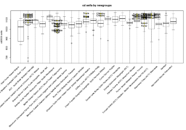
Assess the outliers

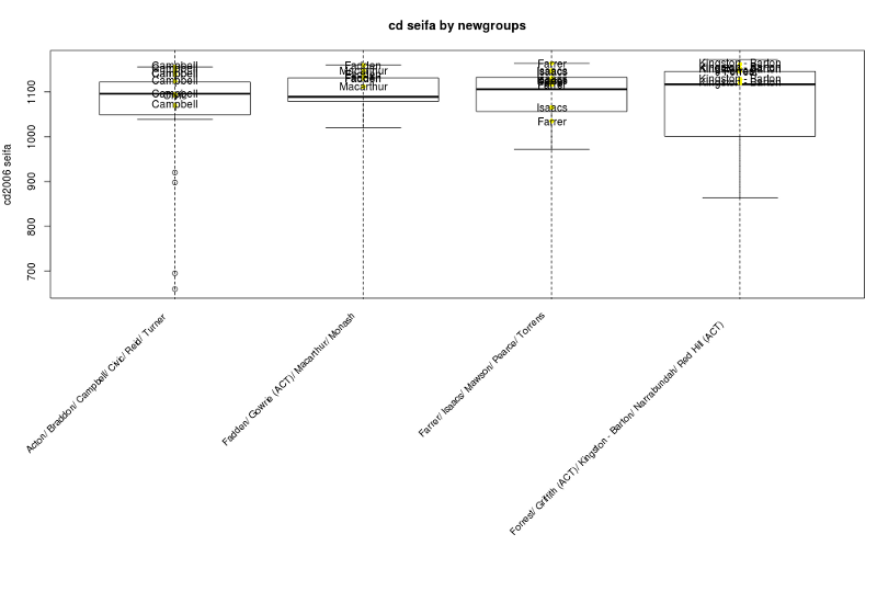
• this can be done by identifying their component CCD SEIFA within new groups
• the seifa of CCD in outliers are compared to the others within their new groups

• zoom in on croweded areas

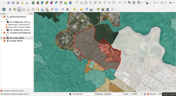
Investigating areas: eg the Kingston - Barton area

• we can zoom in on some of these areas

Conclusions

Basically, the problem comes from public housing policies in Canberra which distorts the effect of the housing market and land values in segregating rich from poor. Essentially, there are highly advantaged suburbs with pockets of disadvantaged public housing.

Other ‘problematic’ features re this are:

• proximity to ornamental lakes
• proximity to urban green space
• proximity to rural residential hubs (walaroo road? hall?). This is a bit of a reverse statement – but different to ‘distance from urban centre’
• elevation, especially with a view.

Potentially the issue is going to be that this can’t be solved if you want to maintain SA2 as the base level - the distinctions are going to be at an SA1 or even mesh block level.