Welcome to my Open Notebook

This is an Open Notebook with Selected Content - Delayed. All content is licenced with CC-BY. Find out more Here.

ONS-SCD.png

Templates are Needed for Reproducible Research Reports (that Look Good)

I read with interest the the Transparency and Openness Promotion (TOP) Committee templates for guidelines to enhance transparency in the science that journals publish.

Citation

Supplementary Materials for Nosek, B. A., Alter, G., Banks, G. C.,
Borsboom, D., Bowman, S. D., Breckler, S. J., … Yarkoni,
T. (2015). Promoting an open research culture. Science, 348(6242),
1422–1425. doi:10.1126/science.aab2374

I think though that guidelines like the suggestion to copy-paste bits of the manuscript leave a bit to be desired:

Quote;

Authors document compliance by copy-pasting the relevant passages
in the paper that address the question into the form. For example,
when indicating how sample size was determined, authors copy paste
into the form the text in the paper that describes how sample size
was determined.

Reproducible Research Reports solve this problem by ensuring that the data preparation and analysis are executed in the same script that produces the manuscript, therefore a one-stop-shop for documentation of the entire study.

There is a need for Templates of Reproducible Research Reports (that look good!)

Rstudio provides very easy support for these documents if you use R. In particular the option of a menu button to create a new report populates that report with the required header information and some example script to work off. But the easiest option does not look so good. This is the Rmarkdown option and it is very user friendly in terms of the markup language needed to write the descriptive language around your analysis (mostly plain text with a few simple options for heading styles etc) rather than the Sweave option which leads to the full blown LaTeX markup language that is a lot more complicated.

Boilerplate Rmarkdown header from Rstudio:

---
title: "Untitled"
author: "Ivan C. Hanigan"
date: "16 September 2015"
output: html_document
---

This is great for quick reporting of work as you go, but I primarily write for output that will be printed (e.g. pdf docs). More specifically, I need the concept of a page, and to have full control over the placement of table and figure ‘environments’, stuff that is easy in LaTeX (once you figure out some of the esoteric parts of that language).

To achieve a simple writing environment in Markdown but with the powerful layout options of LaTeX I reviewed this guys work but I think it takes it to an uneccessary level of complicated-ness https://github.com/jhollist/manuscriptPackage.

So I went back to some of the old Sweave/Latex templates I had put together and ported it into a markdown header.

Boilerplate Rmarkdown header for pretty report

---
title: "Untitled"
author: "Ivan C. Hanigan"
date: "16 September 2015"
header-includes:
  - \usepackage{graphicx}
  - \usepackage{fancyhdr} 
  - \pagestyle{fancy} 
  - \usepackage{lastpage}
  - \usepackage{float} 
  - \floatstyle{boxed} 
  - \restylefloat{figure} 
  - \usepackage{url} 
  - \usepackage{color}
  - \lhead{Left Header}
  - \chead{Rmarkdown Rocks}
  - \rhead{\today}
  - \lfoot{Left Footer}
  - \cfoot{Centre Footer}
  - \rfoot{\thepage\ of \pageref{LastPage}}  
output: 
  pdf_document:
    toc: false
documentclass: article
classoption: a4paper
bibliography: references.bib
---

Now the layout of tables and figures is done with latex

Code

Using the xtable package allows results to be displyed in tables
and has built in support for some R objects, so summrising the
linear fit above in ~\ref{ATable}
  
```{r, results='asis', type = 'tex'}
library(xtable)    
print(xtable(fit, caption="Example Table",
  digits=4,table.placement="ht",label="ATable"), comment = F)    
```
   
## A Plot
   
Plots intergrate most easily if made seperately as can be seen in figure ~\ref{test}
```{r}
png("Rmarkdownfig.png")
plot(x,y,main="Example Plot",xlab="X Variable",ylab="Y Variable")
abline(fit,col="Red")
dev.off()
```
\begin{figure}[H]
\begin{center}
\includegraphics[width=.5\textwidth]{Rmarkdownfig.png}
\end{center}
\caption{Some Plot}
\label{test}
\end{figure}
\clearpage

I also realised that if this was to be a full report of a scientific study it would need to include some of the machinery needed for bibliographies.

Stuff for bibliographies

```{r, echo=F, results = 'hide', message = F, warning=F}
library("knitcitations")
library("bibtex")
cleanbib()
cite_options(citation_format = "pandoc", check.entries = FALSE)
 
bib <- read.bibtex("C:/Users/Ivan/Dropbox/references/library.bib")
 
```

<!--Put data analysis and reporting here, then at the end of the doc-->

```{r, echo=F, message=F, eval=T}
write.bibtex(file="references.bib")
```
      
# References

<!--The bib will then be written following the final subheading-->

Conclusion

I hope this might help others develop their own templates for RRR that look great.

Posted in  disentangle reproducible research reports


task-management-like-an-open-science-hacker

I just read this impressive paper and it has really given me a push toward making this open lab notebook

Citation

Nosek, B. A., et al. (2015). Promoting an open research
culture. Science, 348(6242), 1422–1425. doi:10.1126/science.aab2374

Quote

The situation is a classic collective action problem. Many individual researchers lack
strong incentives to be more transparent, even though the credibility of science would 
benefit if everyone were more transparent.

So I think I’ll try to step up the pace of logging my daily scientific work. One super easy thing to do is to publish my daily log from my task management in orgmode. Indeed I am also reading at the moment this guy who says

Quote

The core of your documentation is the research log.
   
Long, S. (2015). Reproducible Results and the Workflow of Data Analysis. 
Retrieved from http://www.indiana.edu/~jslsoc/ftp/WIM/wf wim 2015 2015-08-21@3.pdf

Finally, I was struck by this reference http://rich-iannone.github.io/about/2014/10/28/introduction.html to something about 365+ day GitHub streaks. It was covered earlier by Geoff Greer, and by Dirk Eddelbuettel.

It seems the basic concept is that you can leverage off an obsessive tendency by making sure you do something toward ticking off items from the task list every day. The impulse to not breaking the chain is supposed to give you inspiration to keep going. I think this might work well for my temperatment.

Emacs and orgmode

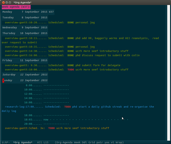
The set up of my daily log is pretty simple. After being set up by kjhealy’s starter kit. Then I modified the org-agenda-files which was set in the main el file that kjhealy provided and then with the command C-c a a emacs will display my calendar.

When I open emacs in the morning I open the agenda and this also opens research-log file. I move to that buffer, then I use this key command to insert a new entry for todays date

CODE

 (define-skeleton org-journalentry
   "Template for a journal entry."
   "project:"
   "*** " (format-time-string "%Y-%m-%d %a") " \n"
   "**** TODO-list \n"
   "***** TODO \n"
   "**** timesheet\n"
   "#+begin_src txt :tangle work-log.csv :eval no :padline no\n"
   (format-time-string "%Y-%m-%d %a") ", " str ", 50\n" 
   "#+end_src\n"
 )
 (global-set-key [C-S-f5] 'org-journalentry)

This creates a new date, a stub of a TODO for anything ad hoc and a entry into my timesheet.csv file.

I then select from TODO items from a global list that I keep at the top of the file, and cut/paste them into todays list.

img

Great so I just moved this research-log orgmode file into my blog github repo, and with the help of charlie park’s bash script I am good to go

CODE

alias build_blog="cd ~/projects/ivanhanigan.github.com.raw; jekyll b;
cp -r ~/projects/ivanhanigan.github.com.raw/_site/* ~/projects/ivanhanigan.github.com;
cd ~/projects/ivanhanigan.github.com;git add .;git commit -am 'Latest build.';git push"
alias bb="build_blog"

So this will put the resulting changes onto my open lab book website here https://raw.githubusercontent.com/ivanhanigan/ivanhanigan.github.com/master/work-log.org

Things to note:

  • I found this list of tips http://natashatherobot.com/streak-github-mistakes/
  • In particular I realise I need to make my daily push by 4:50 PM in Canberra ACT as this is 11:50 PM the previous day for Github, Pacific Time (PT)
  • I also will need to ensure I don’t publish sensitive (or embarrasing entries).
  • I’ll try to keep the identity of my collaborators private as well, so just use their initials rather than names.

Posted in  disentangle


how-to-say-why-before-what

I have discovered a flaw in my writing style.
I often say what it it before I say why it is important.

Example

Disentangling health effects of environmental from social factors
is difficult for a variety of reasons. The effort to examine and
to separate environmental and social causes is nevertheless
valuable. [WHY IS IT VALUABLE?] This is especially important to
policy makers and to others who seek to maximise the public
good. A greater understanding of their respective contributions
will lead to more rational, deep-seated, lasting and effective
interventions.

The caps question is from someone reading my draft. I need to start with the why. Perhaps just turn the paragraph on its head?

Example

A greater understanding of the respective contributions from
environmental and social factors will lead to more rational,
deep-seated, lasting and effective interventions by policy makers
and to others who seek to maximise the public good.  Disentangling
health effects of environmental from social factors is difficult
for a variety of reasons. The effort to examine and to separate
environmental and social causes is nevertheless valuable.

Posted in  disentangle


tracking-a-data-analysis-pipeline

I have just uploaded a new version of the windows build for my ‘disentangle’ package. The blurb of the draft vignette is below.

Introduction

It can be much easier to conceptually understand a complicated data analysis pipeline than it is to implement that pipeline effectively. This report outlines the use of the ‘disentangle’ R package, available from http://ivanhanigan.github.io/projects.html. This package contains functions that were developed to aid data analysts to map out all the aspects of their work when planning and conducting complicated data analyses using the pipeline concept. There are often many steps in the design and analysis of a study and when these are put together as a data analysis pipeline this addresses the challenge of reproducibility (Peng 2006). The credibility of data analyses requires that every step is able to be scrutinised (Leek 2015).

Motivating scientific questions

The type of data analysis that is the focus of this work is more complicated than simply loading some data that are already cleaned, fitting some models and reporting some output. Typically the type of data analysis projects that these tools are aimed at involve attempts to control for a large number of inter-relationships and associations between variables. It is especially problematic that these variables need to have been selected by the scientists from a multitude of possible variables and a plethora of possible data sources, during a long process of data collection, cleaning, exploration and decision making in preparation for data analysis. There are also a multitude of steps and decision points in the process of model building and model checking. The use of statistical models involving many entangled environmental and social variables can easily result in spurious association that may be mistakenly interpreted as causation. Projects that the author has been involved in include explorations of hypotheses about health effects from droughts, bushfire smoke, heat-waves and dust-storms which produced novel findings, and informed controversial debates about the implications of climate change. The requirement to adequately convey the methods and results of this research was problematic and motivated the work on effective use of reproducible research techniques and data analysis pipelines.

Posted in  disentangle


Web Data, Climate Grids and THREDDS UPDATE

Update

QUOTE:

"you need to use ncdf4  - not ncdf  ...
because they are netcdf4 files and not netcdf3 files. 
This is poorly explained in the R community.
All of the netcdf files from Australian providers (AusCover, BoM, etc...) 
have been in netcdf4 for a couple of years now."

So here is the revised code using ncdf4 library:

CODE

# sudo apt-get install r-cran-ncdf4 
library(ncdf4)
library(raster)
strt <-'2012-01-01'
end <- '2012-01-04'
dates <- seq(as.Date(strt),as.Date(end),1)          
dates
par(mfrow = c(2,2))
for(i in 1:length(dates)){
 # i=1
  date_i <- dates[i]
  infile <- sprintf("http://dapds00.nci.org.au/thredds/dodsC/rr9/Climate/eMAST/ANUClimate/0_01deg/v1m0_aus/day/land/tmin/e_01/2012/eMAST_ANUClimate_day_tmin_v1m0_%s.nc", gsub("-", "", date_i))
 
  nc <- nc_open(infile)
  str(nc)
  print(nc)
  vals <- ncvar_get(nc, varid="air_temperature")
  str(vals)
  nc.att <-    nc$var$air_temperature
  xmin <- min(nc.att$dim[[1]]$vals)
  xmax <- max(nc.att$dim[[1]]$vals)
  ymin <- min(nc.att$dim[[2]]$vals)
  ymax <- max(nc.att$dim[[2]]$vals)
 
  print(c(xmin,xmax))
  print(c(ymin,ymax))
 
  r <- raster(t(vals),
              xmn=xmin, xmx=xmax,
              ymn=ymin, ymx=ymax)
  #str(r)
  plot(r)
  nc_close(nc)
}

RESULTS 1: METADATA

  • the result is I now have a lot more metdata returned to my R workspace

EXERPT

[...]
[1] "        licence_copyright: Copyright 2009-2013 ANU. Rights owned by The Australian National University (ANU). Rights licensed subject to TERN  Attribution (TERN-BY)."
[1] "        short_desc: Australian coverage, ANUClimate 1.0, 0.01 degree grid, 1970-2012"
[1] "        summary: Minimum daily temperature, for the Australian continent between 1970-2012. Daily temperature regulates rates of plant growth and determines critical conditions such as frost on flowering and fruiting. Modelled by expressing each daily value as a difference anomaly with respect to the gridded 1976-2005 mean daily minimum temperature for each month as provided by eMAST_ANUClimate_mmn_tmin_v1m0_1976_2005. The daily anomalies were interpolated by trivariate thin plate smoothing spline functions of longitude, latitude and vertically exaggerated elevation using ANUSPLIN Version 4.5. There was an average of 671 Bureau of Meteorology data points available for each day between 1970 and 2012. Automated quality assessment rejected on average 3 data values per day with extreme studentised residuals. These were commonly associated with days following missing observations. The root mean square of all individual cross validation residuals provided by the spline analysis is 1.5 degrees Celsius. A comprehensive assessment of the analysis and the factors contributing to the quality of the final interpolated daily minimum temperature grids is in preparation."
[1] "        long_name: Daily minimum temperature"
[1] "        contact: Michael Hutchinson, Professor of spatial and temporal analysis, 3.23A, Fenner School of Environment & Society, College of Medicine, Biology & Environment, Frank Fenner Building 141, Australian National University, Canberra, Australian Capital Territory, 200, Australia, (+61) 2 6125 4783, Michael.Hutchinson@anu.edu.au, http://orcid.org/0000-0001-8205-6689"
[1] "        references: 1. Hutchinson, M.F., Mckenney, D.W., Lawrence, K., Pedlar, J., Hopkinson, R., Milewska, E. and Papadopol, P. 2009. Development and testing of Canada-wide interpolated spatial models of daily minimum/maximum temperature and precipitation for 1961-2003. Journal of Applied Meteorology and Climatology 48: 725�741. http://dx.doi.org/10.1175/2008JAMC1979.1 2. Hutchinson, M.F. and Xu, T. 2013. ANUSPLIN version 4.4 User Guide. Fenner School of Environment and Society, Australian National University, Canberra http://fennerschool.anu.edu.au/files/anusplin44.pdf"
[1] "        source: ANUClimate 1.0"
[1] "        keywords: EARTH SCIENCE > ATMOSPHERE > ATMOSPHERIC TEMPERATURE > MAXIMUM/MINIMUM TEMPERATURE"
[1] "        Conventions: CF-1.6"
[1] "        institution: Australian National University"
[1] "        geospatial_lat_min: -43.74"
[1] "        geospatial_lat_max: -9"
[1] "        geospatial_lat_units: degrees_north"
[1] "        geospatial_lat_resolution: -0.01"
[1] "        geospatial_lon_min: 112.9"
[1] "        geospatial_lon_max: 154"
[1] "        geospatial_lon_units: degrees_east"
[1] "        geospatial_lon_resolution: 0.01"
[1] "        keywords_vocabulary: Global Change Master Directory (http://gcmd.nasa.gov)"
[1] "        metadata_link: http://datamgt.nci.org.au:8080/geonetwork"
[1] "        standard_name_vocabulary: Climate and Forecast(CF) convention standard names (http://cf-pcmdi.llnl.gov/documents/cf-standard-names)"
[1] "        id: eMAST_ANUClimate_day_tmin_v1m0_1970_2012"
[1] "        DOI: To be added"
[1] "        cdm_data_type: grid"
[1] "        contributor_name: Michael Hutchinson, Jennnifer Kesteven, Tingbao Xu"
[1] "        contributor_role: principalInvestigator, author, author"
[1] "        creator_email: eMAST.data@mq.edu.au"
[1] "        creator_name: eMAST data manager"
[1] "        creator_url: http://www.emast.org.au/"
[1] "        Metadata_Conventions: Unidata Dataset Discovery v1.0"
[1] "        publisher_name: Ecosystem Modelling and Scaling Infrastructure (eMAST) Facility: Macquarie University"
[1] "        publisher_email: eMAST.data@mq.edu.au"
[1] "        publisher_url: http://www.emast.org.au/"

RESULTS 2: Grid data

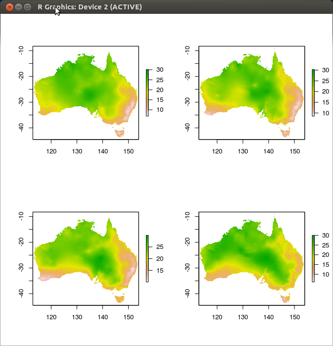
  • I still get lots of good data

/images/thredds2.png

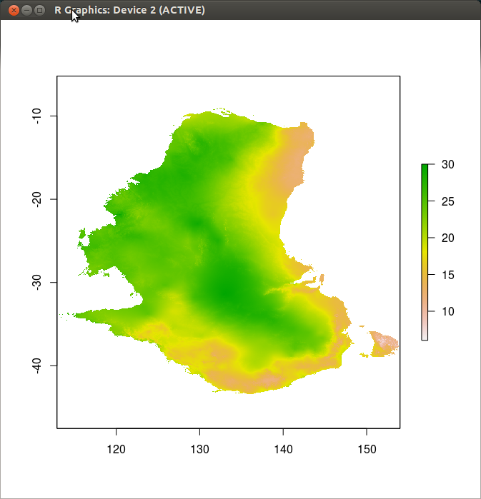
NOTE I still need that weird transpose

  • I note that the weird hacky transpose is still required

CODE

# NB weird hacky transpose still required or else you get this
r <- raster(vals,
            xmn=xmin, xmx=xmax,
            ymn=ymin, ymx=ymax)
 
#str(r)
plot(r)

/images/thredds2raw.png

Posted in  extreme weather events