require(devtools)
install_github("gisviz", "ivanhanigan")
require(gisviz)
require(swishdbtools)
ch <- connect2postgres2("gislibrary")
# make a temporary tablename, to avoid clobbering
temp_table <- swish_temptable("gislibrary")
temp_table <- paste("public", temp_table$table, sep = ".")
temp_table
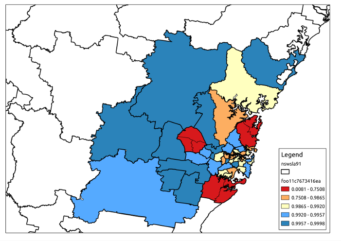
# this is going to be public.foo11c7673416ea
sql <- postgis_concordance(conn = ch, source_table = "abs_sla.nswsla91",
source_zones_code = 'sla_id', target_table = "abs_sla.nswsla01",
target_zones_code = "sla_code",
into = temp_table, tolerance = 0.01,
subset_target_table = "cast(sla_code as text) like '105%'",
eval = F)
cat(sql)
dbSendQuery(ch, sql)
dbSendQuery(ch, sprintf("drop table %s", temp_table))