
- today I was in a meeting where the discussion turned to maps of crude incidence rates, age-standardised rates and regression models controlling for age
- If disease incidence does not vary with age then there is not much point in controlling for this,
- apart from the work done in exploratory data analysis to ascertain whether or not this is the case
- I proposed that if you’ve done all the work on age-specific rates needed to test if incidence varies with age, then you might as well present age adjusted rates seeing as you’ve already done the work anyway
An example
- The project is highly confidential due to the nature of the data
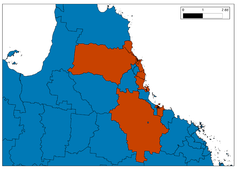
- We;ll call the study location South Kingsland to protect the identity
R Code:
# get spatial data
require(swishdbtools) # github package, under
                      # swish-climate-impact-assessment

Tab1 <- read.csv("data/dataset.csv", sep= ",", header = TRUE, stringsAsFactor = F)
Tab1 <- as.data.frame(table(Tab1$SLA))
nrow(Tab1)
write.csv(Tab1, "data/SLA.csv", row.names = F)
load2postgres("data/SLA.csv", schema="ivan_hanigan", tablename="sla", ip = "brawn.anu.edu.au",
              db = "gislibrary", pguser = "ivan_hanigan", printcopy = F)


ch  <- connect2postgres2("gislibrary")
sql_subset(ch, "ivan_hanigan.sla", eval = T, limit = 10)


sql_subset(ch, "abs_sla.qldsla01", select =  "sla_name, st_y(st_centroid(geom))", eval = T, limit = 10)
dbSendQuery(ch,
  "select sla_name, geom
  into southkingsland
  from abs_sla.qldsla01 t1
  join
  sla t2
  on t1.sla_name = t2.var1;
  alter table southkingsland add column gid serial primary key;
  ")
# these are missing from spatial data
## 42                      West End                          <NA>
## 43                OVERSEAS-OTHER                          <NA>
## 44                  Yarrabah (S)                          <NA>
## 45     Rowes Bay-Belgian gardens                          <NA>
visualise with QGIS
R Code:
# func
require(plyr)

# load
Tab2 <- read.csv("data/dataset.csv", sep= ",", header = TRUE, stringsAsFactor = F)
names(Tab2)
# [1] "SLA"       "agegrp"    "Sex"       "district"  "dm"        "ninf"
# [7] "popSLA"    "Month"     "Year"      "groupyear"
test_sla  <- names(table(Tab2$SLA)[1])
subset(Tab2, SLA == test_sla & Year == 2001 & agegrp == 1 & Sex == "MALE")
subset(Tab2, SLA == test_sla & Year == 2001 & agegrp == 1 & Sex == "FEMALE")

# clean
summary(Tab2)
## remove any SLA with NA populations
Tab2 <- Tab2[which(!is.na(Tab2$popSLA)),]

# do
## first total cases by annualised pop
analyte  <- ddply(Tab2, c("SLA", "Year", "agegrp", "Sex"), summarise,
                  ninf=sum(ninf),
                  popSLA=mean(popSLA)
                  )
#str(analyte)

#subset(analyte, SLA == test_sla)
subset(analyte, SLA == test_sla & Year == 2001 & agegrp == 1)

## now annual totals for study region
analyte2  <- ddply(analyte, c("Year", "agegrp"), summarise,
                  ninf=sum(ninf),
                  popSLA=sum(popSLA)
                  )
str(analyte2)

qc <- subset(analyte2,  Year == 2001)
qc
sum(qc$popSLA)

## now totals
qc  <- ddply(analyte2, c("Year"), summarise,
             ninf=sum(ninf),
             popSLA=sum(popSLA)
             )
qc
sum(qc$ninf)
mean(qc$popSLA)

## totals by age
subset(analyte2,  agegrp == 1)
analyte3  <- ddply(analyte2, c("agegrp"), summarise,
                  ninf=sum(ninf),
                  popSLA=mean(popSLA)
                  )
analyte3
sum(analyte3$popSLA)
analyte3$asr  <- (analyte3$ninf / analyte3$popSLA) * 1000
analyte3

png("graphs/south-kingsland-age-specific-rates.png")
mp <- barplot(analyte3$asr, names.arg = analyte3$agegrp)
box()
dev.off()
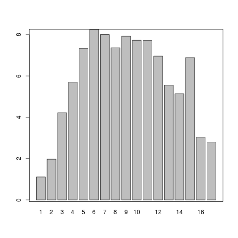
Plot Age Specific Rates
Great so with that bit of work we should have an idea of the variation of incidence by age
Results and Discussion
- It looks like the incidence does vary with age
- TODO make graphs per year (the scale of the above graph is wrong - decades in the numerator but annualised pops in the denominator)
- TODO make graphs by city, by sex
- age-standardised rates probably need different age categories, only 4 or 5?
- worth commenting on the liklihood that age is not important for time-series models at the city scale, unless age structure changes substantially over time (this is an analysis for the spatial pattern only)
Clean up database!
dbSendQuery(ch, "drop table sla")
dbSendQuery(ch, "drop table southkingsland")


