This is a great example of logistic regression, because it is pretty simple but covers good ground. I got it from Peter Caley;s R tutorial workbook from Charles Darwin School of Environmental Research.
It is also a tragic example of the impact weather can have on health.
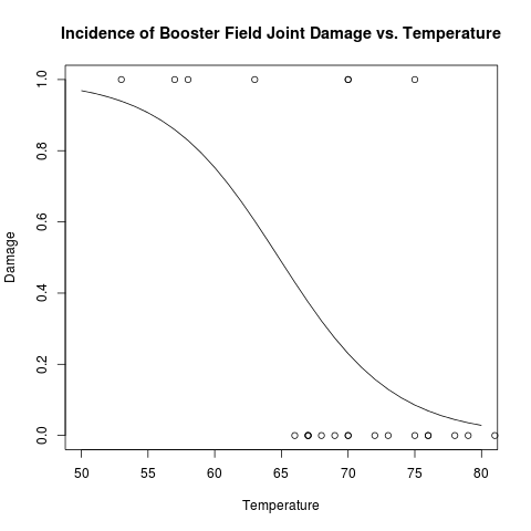
The colder it is the more likely the shuttle is to explode.
The problem was with the failure rate (and number of) O-rings that failed (n.fail) related to the temperature (temp).
R Code:
#Load the data
#The following R code will construct the dataset
n.fail <- c(2, 0, 0, 1, 0, 0, 1, 0, 0, 1, 2, 0, 1, 0, 0, 0, 0, 0, 1, 0, 0, 0, 0)
temp <- c(53, 66, 68, 70, 75, 78, 57, 67, 69, 70, 75, 79, 58, 67, 70, 72, 76, 81, 63, 67, 70, 73, 76)
# there were 6 o rings for each of 23 attempts
total <- rep(6,23)
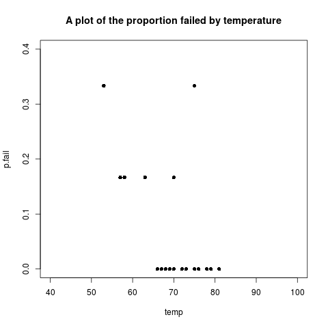
# probability of fail
p.fail <- n.fail/total
# Response = resp column bind them together
resp <- cbind(n.fail, total-n.fail)
###########################################################################
# we can write text files easily once the data frame or matrix is in shape
data <- as.data.frame(cbind(resp,temp))
names(data) <- c('nfail','totalMinusNfail', 'temp')
# write.csv(data, 'learnR-logistic-data.csv', row.names=F)
###########################################################################
# and read it in again
# data2 <- read.csv('learnR-logistic-data.csv')
################################################################
# name:learnR-logistic
png('images/pfail.png')
plot(temp, p.fail, pch=16, xlim=c(40,100), ylim=c(0,0.4))
title('A plot of the proportion failed by temperature')
dev.off()
R Code:
###########################################################################
# newnode: linear
linear <- glm(resp ~ 1 + temp, family=binomial(link=logit))
summary(linear)
linearoutput <- summary(linear)
linearoutput$coeff
###########################################################################
# newnode: learnR-logistic
cf <- linearoutput$coeff
signif(cf[which(row.names(cf) == 'temp'),'Estimate'],2)
###########################################################################
# newnode: learnR-logistic
# write.csv(linearoutput$coeff,"challengerOfails.csv")
###########################################################################
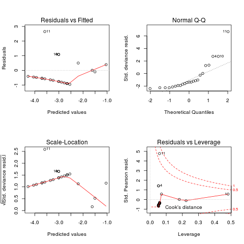
# newnode: learnR-logistic
png('images/challengerLogistic.png')
par(mfrow=c(2,2))
plot(linear)
dev.off()
R Code:
####################################################################
# newnode: learnR-logistic
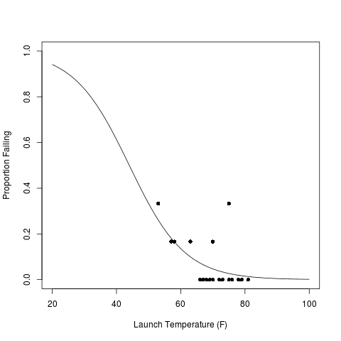
dummy <- data.frame(temp=seq(20,100,1))
pred.prob <- predict.glm(linear, newdata=dummy, type="resp")
png('images/pfailfit.png')
plot(temp, p.fail, xlab="Launch Temperature (F)",
ylab="Proportion Failing", pch=16, xlim=c(20,100), ylim=c(0,1.0))
lines(dummy$temp, pred.prob)
dev.off()
R Code:
####################################################################
resp <- as.data.frame(resp)
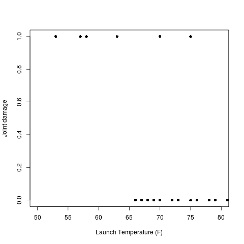
resp$fail <- ifelse(resp$n.fail > 0, 1, 0)
resp$temp <- temp
png('images/fail.png')
with(resp, plot(temp, fail, xlab="Launch Temperature (F)",ylab="Joint damage", pch=16, xlim=c(50,80), ylim=c(0,1.0))
)
dev.off()
R Code:
chal.logit <- glm(fail~temp,family=binomial, data = resp)
summary(chal.logit)$coeff

png('images/pfailfit2.png')
cx <- c(50:80/1)
cyhat <- coefficients(chal.logit)[c(1)] +
coefficients(chal.logit)[c(2)]*cx
cpihat <- exp(cyhat)/(1+exp(cyhat))
with(resp,plot(temp,fail,xlab="Temperature",ylab="Damage",
main="Incidence of Booster Field Joint Damage vs. Temperature", xlim = c(50,80))
     )
lines(cx,cpihat)
dev.off()