Spatiotemporal multilevel modelling

1 Introduction
- 1.1 Overview
2 Compare basic regression with mixed-effects modelling
- 2.1 Terminology
- 2.2 Introduce the linear model and lmer
3 Intercepts and coefficients that vary by group
- 3.1 Ross River virus and urban vs rural mosquito habitat
4 Spatially structured timeseries
5 Spatial lag and timeseries
- 5.1 Data
  - 5.1.1 Zones
  - 5.1.2 Outcome
- 5.2 Analysis
  - 5.2.1 Model with Spatial Lag
  - 5.2.2 Spatial Lag Model Plots

1 Introduction

1.1 Overview

In this notebook we will introduce what multi-level data and models are and why they are useful in epidemiology contexts. We begin with the general linear model framework GLM and then move to mixed-effects models. It is important to realise that these models are called different things in different disciplines: (generalized) linear mixed (effects) models (GLMM), hierarchical (generalized) linear models, etc. The terminology for the model parameters is equally diverse, usually including the terms random effects and fixed effects. So we focus on the key concepts.

We will cover what is a Random Effect and how it differs from a Fixed effect. Some example syntax in R (on a secure website portal we have configured) and Stata will show how to get a handle on models that have random intercepts and additionally, random slopes.

We will spend a little time talking about how to partition variation and get estimates of the random and fixed effects. An important element will be our discussion of similarities between mixed-effects models with basic regression. There will also be brief discussion of extending the regression to non-gaussian responses (GLMERs).

We will discuss how to interpret these results in a population health context.

An online analysis server (Rstudio in a web browser) and data repository (geoserver) are also provided

2 Compare basic regression with mixed-effects modelling

2.1 Terminology

When discussing multilevel modelling in this workshop we will avoid using the names 'fixed effects' and 'random effects'. Instead we use the more verbose phrase: intercepts/coefficients that are common across groups and intercepts/coefficients that vary by group. This is because, as noted in the introduction to Gelman and Hill 2007 (recommended reading) it is very problematic that these terms are used in imprecise and confusing ways that vary across disciplines. This concern also appears in the work of the rstanarm package developers and in the vignette 'Estimating Generalized Linear Models with Group-Specific Terms with rstanarm' who state:

'Models with this structure are referred to by many names: multilevel models, (generalized) linear mixed (effects) models (GLMM), hierarchical (generalized) linear models, etc. The terminology for the model parameters is equally diverse… [and commonly used terms] are not only misleading but also defined differently across the various fields in which these models are applied.'

2.2 Introduce the linear model and lmer

3 Intercepts and coefficients that vary by group

3.1 Ross River virus and urban vs rural mosquito habitat

See do_model_checking_glmer

#########################

4 Spatially structured timeseries

I will use the NMMAPSlite datasets for a simple example of what I describe as "Spatially Structured Timeseries" as opposed to "Spatio-Temporal" which I think more explicitly includes spatial structure in the model.

4.1 Outcome Data

4.1.1 Original Data

"
http://cran.r-project.org/web/packages/NMMAPSlite/index.html
Package ‘NMMAPSlite’ was removed from the CRAN repository.
Formerly available versions can be obtained from the archive.
Archived on 2013-05-11 at the request of the maintainer.

The Archived versions do not seem to work either.

That is such a shame, lucky I saved some of the data using the following code:
"

   
#### Code: get nmmaps data
# func
if(!require(NMMAPSlite)) install.packages('NMMAPSlite');require(NMMAPSlite)

######################################################
# load  
setwd('data')
initDB('data/NMMAPS') # this requires that we connect to the web,
                      # so lets get local copies
setwd('..')
cities <- getMetaData('cities')
head(cities)
citieslist <- cities$cityname
# write out a few cities for access later
for(city_i in citieslist[sample(1:nrow(cities), 9)])
{
 city <- subset(cities, cityname == city_i)$city
 data <- readCity(city)
 write.table(data, file.path('data', paste(city_i, '.csv',sep='')),
 row.names = F, sep = ',')
}
# these are all tiny, go some big ones
for(city_i in c('New York', 'Los Angeles', 'Madison', 'Boston'))
{
 city <- subset(cities, cityname == city_i)$city
 data <- readCity(city)
 write.table(data, file.path('data', paste(city_i, '.csv',sep='')),
 row.names = F, sep = ',')
}

4.1.2 Pooled Dataset

################################################################
# name:Pooled Dataset
setwd("~/projects/spatiotemporal-regression-models/NMMAPS-example")

flist <- dir("data", full.names=T)

flist <-    flist[which(basename(flist) %in%
                        c("Baton Rouge.csv",
                          "Los Angeles.csv",
                          "Tucson.csv",
                          "Denver.csv")
                        )
                  ]
flist
for(f_i in 1:length(flist))
    {
        #f_i <- 2
        fi <- flist[f_i]
        df <- read.csv(fi)
        df <- df[,c("city","date", "agecat",
                    "cvd", "resp", "tmax",
                    "tmin", "dptp")]
        # str(df)
        write.table(df,
                    "outcome.csv", sep = ",",
                    row.names = F, append = f_i > 1,
                    col.names = f_i ==1
                    )
    }

4.2 Exposure Data

4.3 Zones

4.3.1 Map Shapefile Code

################################################################
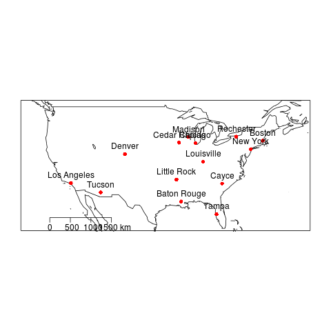
# name:zones
# func
setwd("~/Dropbox/projects/spatiotemporal-regression-models/NMMAPS-example")
#require(devtools)
#install_github("gisviz", "ivanhanigan")
require(gisviz)

# load
flist <- dir("data")
flist
# do    
## geocode
flist <- gsub(".csv", "", flist)    
flist_geo <- gGeoCode2(flist)
flist_geo

## plot
## png("images/nmmaps-eg-cities.png")
## plotMyMap(
##     flist_geo[,c("long","lat")],
##     xl = c(-130,-60), yl = c(25,50)
##     )
## text(flist_geo$long, flist_geo$lat, flist_geo$address, pos=3)
## dev.off()
   
# load city names
flist2 <- dir("data")
flist2
city_codes <- matrix(NA, nrow = 0, ncol = 2)
for(fi in 1:length(flist2))
    {
        # fi <- 1
        fname <- flist2[fi]
        print(fi); print(fname);
        df <- read.csv(
            file.path("data", fname),
            stringsAsFactors = F, nrow = 1)
        city_codes <- rbind(city_codes,
            c(gsub(".csv","",fname), df$city)
            )
    }
city_codes <- as.data.frame(city_codes)
names(city_codes) <- c("address","city")
city_codes 
flist_geo2 <- merge(flist_geo, city_codes, by = "address")
flist_geo2

## make shapefile
epsg <- make_EPSG()
prj_code <- epsg[grep("WGS 84$", epsg$note),]
prj_code
shp <- SpatialPointsDataFrame(cbind(flist_geo2$long,flist_geo2$lat),flist_geo2,
                              proj4string = CRS(
                                  epsg$prj4[which(epsg$code ==prj_code$code)]
                                  )
                              )
writeOGR(shp, 'cities.shp', 'cities', driver='ESRI Shapefile')

4.3.2 Map Shapefile 2

4.3.3 Map Shapefile Output

NMMAPS-example/images/nmmaps-eg-cities.png

4.4 Population Data

4.4.1 Population data

A Code Skeleton
The process for getting the population data from the websites is a bit of a pain, with repeated copy and paste operations. To make sure this is recorded I set up a skeleton to paste into.

TODO better to use gsub() to remove the ","

################################################################
# name:population-data

# func
setwd("~/projects/spatiotemporal-regression-models")
require(gisviz)

# load
## citycodes
shp <- readOGR("cities.shp", "cities")
shp@data
cityname <- "SELECTED CITY"

# do
# save url
# xxx
population_input <- read.table(textConnection(
"age: population
xxx
"), sep = ":", header = TRUE)

## agecats
## 65to74     75p under65  
population_input$agecat <- c(rep("under65", 10),
                             rep("65to74"),
                             rep("75p",2)
                             )

citycode <- subset(shp@data, address == cityname,
                   select = city)

population_input$city <- rep(
    as.character(citycode[1,1])        
    , 13
    )

population_input
if(exists("population"))
    {
        population <- rbind(population,
                            population_input
                            )        
    } else {
        population <- population_input
    }

Baton Rouge

################################################################
# name:population-data
# first city, remove population data.frame
rm(population)

# func
setwd("~/projects/spatiotemporal-regression-models")
require(gisviz)

# load
## citycodes
shp <- readOGR("cities.shp", "cities")
shp@data
cityname <- "Baton Rouge"

# do
# save url
# http://www.city-data.com/us-cities/The-South/Baton-Rouge-Population-Profile.html
population_input <- read.table(textConnection(
"age: population
Population Under 5 years: 15502
Population 5 to 9 years: 15609
Population 10 to 14 years: 15248
Population 15 to 19 years: 21954
Population 20 to 24 years: 27230
Population 25 to 34 years: 31719
Population 35 to 44 years: 30343
Population 45 to 54 years: 27166
Population 55 to 59 years: 9495
Population 60 to 64 years: 7490
Population 65 to 74 years: 13312
Population 75 to 84 years: 9611
Population 85 years and over: 3139
"), sep = ":", header = TRUE)

## agecats
## 65to74     75p under65  
population_input$agecat <- c(rep("under65", 10),
                             rep("65to74"),
                             rep("75p",2)
                             )

citycode <- subset(shp@data, address == cityname,
                   select = city)

population_input$city <- rep(
    as.character(citycode[1,1])        
    , 13
    )

population_input
if(exists("population"))
    {
        population <- rbind(population,
                            population_input
                            )        
    } else {
        population <- population_input
    }

Los Angeles

################################################################
# name:population-data

# func
#setwd("~/projects/spatiotemporal-regression-models")
#require(gisviz)

# load
## citycodes
shp <- readOGR("cities.shp", "cities")
shp@data
cityname <- "Los Angeles"

# do
# save url
# http://www.city-data.com/us-cities/The-West/Los-Angeles-Population-Profile.html
population_input <- read.table(textConnection(
"age: population
Population under 5 years old: 285976
Population 5 to 9 years old: 297837
Population 10 to 14 years old: 255604
Population 15 to 19 years old: 251632
Population 20 to 24 years old: 299906
Population 25 to 34 years old: 674098
Population 35 to 44 years old: 584036
Population 45 to 54 years old: 428974
Population 55 to 59 years old: 143965
Population 60 to 64 years old: 115663
Population 65 to 74 years old: 18711
Population 75 to 84 years old: 125829
Population 85 years and over: 44189
"), sep = ":", header = TRUE)

## agecats
## 65to74     75p under65  
population_input$agecat <- c(rep("under65", 10),
                             rep("65to74"),
                             rep("75p",2)
                             )

citycode <- subset(shp@data, address == cityname,
                   select = city)

population_input$city <- rep(
    as.character(citycode[1,1])        
    , 13
    )

population_input
if(exists("population"))
    {
        population <- rbind(population,
                            population_input
                            )        
    } else {
        population <- population_input
    }

Tucson

################################################################
# name:population-data

# func
#setwd("~/projects/spatiotemporal-regression-models")
#require(gisviz)

# load
## citycodes
shp <- readOGR("cities.shp", "cities")
shp@data
cityname <- "Tucson"

# do
# save url
# http://www.city-data.com/us-cities/The-West/Tucson-Population-Profile.html
population_input <- read.table(textConnection(
"age: population
Population under 5 years old: 35201
Population 5 to 9 years old: 34189
Population 10 to 14 years old: 31939
Population 15 to 19 years old: 38170
Population 20 to 24 years old: 47428
Population 25 to 34 years old: 76394
Population 35 to 44 years old: 72289
Population 45 to 54 years old: 57608
Population 55 to 59 years old: 19597
Population 60 to 64 years old: 16056
Population 65 to 74 years old: 29117
Population 75 to 84 years old: 21394
Population 85 years and older: 7317
"), sep = ":", header = TRUE)

## agecats
## 65to74     75p under65  
population_input$agecat <- c(rep("under65", 10),
                             rep("65to74"),
                             rep("75p",2)
                             )

citycode <- subset(shp@data, address == cityname,
                   select = city)

population_input$city <- rep(
    as.character(citycode[1,1])        
    , 13
    )

population_input
if(exists("population"))
    {
        population <- rbind(population,
                            population_input
                            )        
    } else {
        population <- population_input
    }

Denver

################################################################
# name:population-data

# func
#setwd("~/projects/spatiotemporal-regression-models")
#require(gisviz)

# load
## citycodes
shp <- readOGR("cities.shp", "cities")
shp@data
cityname <- "Denver"

# do
# save url
# http://www.city-data.com/us-cities/The-West/Denver-Population-Profile.html

population_input <- read.table(textConnection(
"age: population
Population under 5 years old: 37769
Population 5 to 9 years old: 34473
Population 10 to 14 years old: 31315
Population 15 to 19 years old: 32259
Population 20 to 24 years old: 45534
Population 25 to 34 years old: 113676
Population 35 to 44 years old: 86420
Population 45 to 54 years old: 71000
Population 55 to 59 years old: 22573
Population 60 to 64 years old: 17191
Population 65 to 74 years old: 30643
Population 75 to 84 years old: 23369
Population 85 years and over: 8414
"), sep = ":", header = TRUE)

## agecats
## 65to74     75p under65  
population_input$agecat <- c(rep("under65", 10),
                             rep("65to74"),
                             rep("75p",2)
                             )

citycode <- subset(shp@data, address == cityname,
                   select = city)

population_input$city <- rep(
    as.character(citycode[1,1])        
    , 13
    )

population_input
if(exists("population"))
    {
        population <- rbind(population,
                            population_input
                            )        
    } else {
        population <- population_input
    }

Louisville

################################################################
# name:population-data

# func
setwd("~/projects/spatiotemporal-regression-models")
require(gisviz)

# load
## citycodes
shp <- readOGR("cities.shp", "cities")
shp@data

cityname <- "Louisville"

# do
# save url
#http://www.city-data.com/us-cities/The-South/Louisville-Population-Profile.html

## NB error in table, 75-84 was missing.  used same from baton rouge
population_input <- read.table(textConnection(
  "age: population
  Population under 5 years old: 16926
  Population 5 to 9 years old: 17359
  Population 10 to 14 years old: 16627
  Population 15 to 19 years old: 17362
  Population 20 to 24 years old: 18923
  Population 25 to 34 years old: 37541
  Population 35 to 44 years old: 40354
  Population 45 to 54 years old: 33755
  Population 55 to 59 years old: 10716
  Population 60 to 64 years old: 9211
  Population 65 to 74 years old: 18577
  Population 75 to 84 years: 9611
  Population 85 years and older: 5075
  "), sep = ":", header = TRUE)

## agecats
## 65to74     75p under65  
population_input$agecat <- c(rep("under65", 10),
                             rep("65to74"),
                             rep("75p",2)
                             )

citycode <- subset(shp@data, address == cityname,
                   select = city)

population_input$city <- rep(
    as.character(citycode[1,1])        
    , 13
    )

population_input
if(exists("population"))
    {
        population <- rbind(population,
                            population_input
                            )        
    } else {
        population <- population_input
    }

Save Population Dataset

################################################################
# name:save-population
write.csv(population, "population.csv",
          row.names = FALSE
          )

4.4.2 Population Summary

################################################################
# name:Population Summary
# func
require(plyr)

# load
population <- read.csv("population.csv")
str(population)
population <- population[,c("city", "agecat", "population")]
# do
population_summary <- ddply(population,
                           .variables = c("city",
                               "agecat"),
                           .fun = summarise,
                           sum(population)
                           )

names(population_summary) <- c("city","agecat","pop")

write.csv(population_summary,
          "population_summary.csv",
          row.names = FALSE
          )

4.5 Merge

################################################################
# name:merge
# func
setwd("~/projects/spatiotemporal-regression-models/NMMAPS-example")

# load
outcome <- read.csv("outcome.csv")
str(outcome)
outcome$date <- as.Date(outcome$date)

population <- read.csv("population_summary.csv")
str(population)
population

# do
analyte <- merge(outcome, population, by = c("city", "agecat"))
analyte <- arrange(analyte, city, date, agecat)
# check
subset(analyte, date == as.Date("1990-01-01"))

# save
write.csv(analyte, "analyte.csv", row.names = FALSE)

4.6 Data Checking

4.6.1 Check Assumption of Proportional Hazards

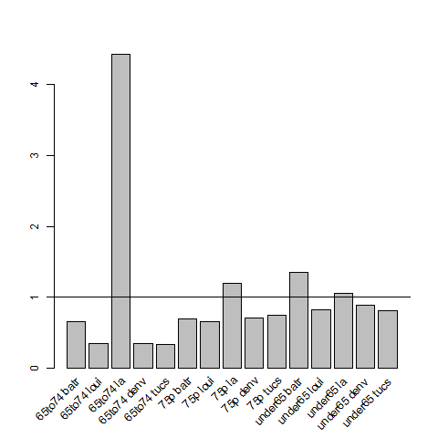
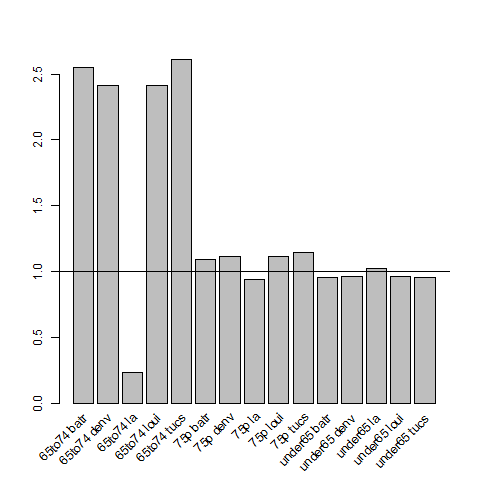
# Checking the proportional hazards assumption for Indirect Age Standardisation

# Background
## Indirect SMRs from different index/study populations are not strictly comparable
## because they are calculated using different weighting schemes that
## depend upon the age structures of the index/study populations
## (see http://www.statsdirect.com/webhelp/#rates/smr.htm).

## Indirect SMRs can be compared if you make the assumption that the
## ratio of rates between index and reference populations is constant;
## this is similar to the assumption of proportional hazards in Cox
## regression (Armitage and Berry, 1994).

## So we need to check if the rate ratio of the study population(s)
## compared to the standard population varies substantially with age.
## If not the proportional hazards assumption holds for the standard
## rates compared with the observed rates and the Indirect SMRs are
## comparable.  To do this check we calculate the Annualised Age Specific
## Rates for our study areas and for our standard for several years at
## periodic timepoints across the study period, and then calculate the
## ratio of these at each timepoint we could reassure our selves that
## this assumption holds.

## An additional issue arises when there are non-negligible differences
## in the age distributions of the study population(s) and the standard
## population. In this situation, indirect standardisation produces
## biased results due to residual confounding by age

## Also see Australian Institute of Health and Welfare. (2011). Principles on
## the use of direct age-standardisation in administrative data
## collections For measuring the gap between Indigenous and
## non-Indigenous Australians. Data linkage series. Cat. no. CSI 12.
## Canberra: AIHW. Retrieved from
## http://www.aihw.gov.au/publication-detail/?id=10737420133

################################################################
# func
setwd("~/projects/spatiotemporal-regression-models/NMMAPS-example")
require(plyr)

# load
analyte <- read.csv("analyte.csv")

# clean
head(analyte)
analyte$yy  <- substr(analyte$date, 1, 4)
  
# do
## first we want to see if the age specific rates vary across the
## study sites
disease_colname <- "cvd"
pop_colname <- "pop"
by_cols  <- c("city", "agecat", "yy")

stdysites  <- ddply(analyte, by_cols,
                    function(df) return(
                      c(observed = sum(df[,disease_colname]),
                        pop = mean(df[,pop_colname]),
                        crude.rate = sum(df[,disease_colname])/mean(df[,pop_colname])
                        )
                      )
                    )
## check
head(stdysites)
subset(stdysites, yy == 1987 & city == "batr")

## define the subset we will use just the deaths and pop in 2000
stdy <- subset(stdysites, yy == 2000)
stdy

## now define the standard population as the entire country
standard  <- ddply(stdy, c("agecat"),
                     function(df) return(
                       c(observed = sum(df[,"observed"]),
                         pop = sum(df[,"pop"]),
                         crude.rate = sum(df[,"observed"])/
                           sum(df[,"pop"])
                         )
                       )
                    )
standard

## Merge the studysites and the standard
stdyByStnd  <- merge(stdy, standard, by = "agecat")
stdyByStnd

## plot the rate ratios
png("images/ratio-stdy-by-stnd.png")
mp <- barplot(stdyByStnd$crude.rate.x/stdyByStnd$crude.rate.y)
text(mp, par("usr")[3],
     labels = paste(stdyByStnd$agecat,stdyByStnd$city),
     srt = 45, adj = c(1.1,1.1), xpd = TRUE
     )
abline(1,0)
dev.off()

## we can see that LA has an issue with the 65to74 agecat

## Second we will check if ratio of the proportions in each population
## agecat vary between study sites and the standard
totals <- ddply(stdyByStnd, c("city"), summarise,
                sum(pop.x)
                )
totals <- merge(stdyByStnd[,c("city","agecat","pop.x")], totals)
totals$pop.wt  <- totals[,3] / totals[,4]
totals <- arrange(totals, city, agecat)
totals

totalsStnd <- ddply(stdyByStnd, c("agecat"), summarise,
                sum(pop.x)
                )
totalsStnd$totalPop <- sum(totalsStnd[,2])
totalsStnd$pop.wt.total <- totalsStnd[,2]/totalsStnd[,3]
totalsStnd

## merge these so we can look at the ratios
totals2 <- merge(totals, totalsStnd, by = "agecat")
totals2 <- arrange(totals2, agecat, city)

## now plot the ratios
png("images/ratio-stdy-by-stnd-pops.png")
mp <- barplot(totals2$pop.wt/totals2$pop.wt.total)
text(mp, par("usr")[3],
     labels = paste(totals2$agecat,totals2$city),
     srt = 45, adj = c(1.1,1.1), xpd = TRUE
     )
abline(1,0)
dev.off()

## and we can see that there are far fewer 65to74 aged persons in LA
## than expected.

4.6.2 Incidence Rate Ratios Plot

NMMAPS-example/images/ratio-stdy-by-stnd.png

4.6.3 Population Rate Ratios Plot

NMMAPS-example/images/ratio-stdy-by-stnd-pops.png

4.7 Exploratory Data Analyses

4.7.1 Time-series Plots Code

################################################################
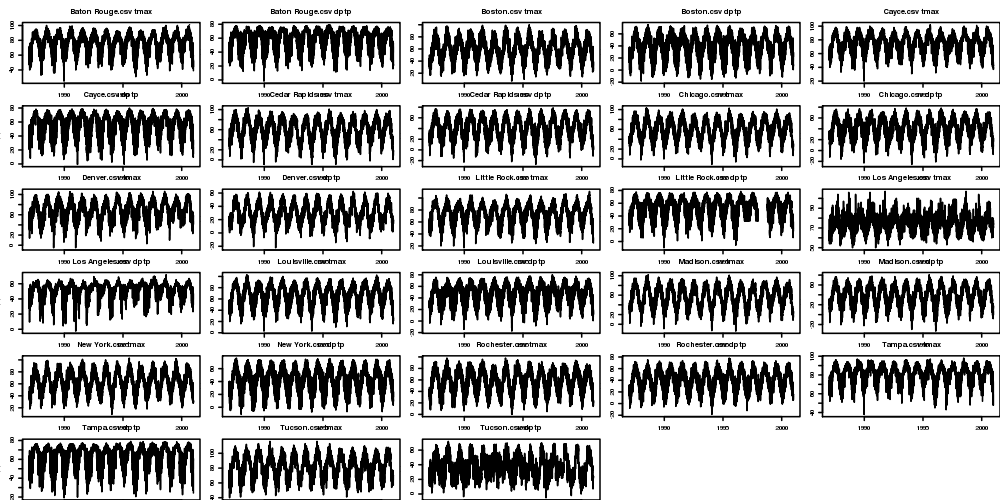
# name:eda-tsplots
# func
setwd("~/projects/spatiotemporal-regression-models/NMMAPS-example")
  
# load
flist <- dir("data")
fname <- flist[7]; print(fname)
df <- read.csv(file.path("data", fname))

# clean
str(df)
summary(df$tmax); summary(df$dptp)

# do
## we will only consider cities with long periods temp and humidity observed
png("images/nmmaps-eg-dateranges.png", width = 1000, height=500, res = 150)
par(mfrow=c(6,5), mar=c(0,3,3,0), cex=.25)
for(fi in 1:length(flist))
    {
        #fi <- 4
        fname <- flist[fi]
        df <- read.csv(file.path("data", fname))
        print(fi); print(fname);
        with(df, plot(as.Date(date), tmax, type = "l"))
        title(paste(fname, "tmax"))
        with(df, plot(as.Date(date), dptp, type = "l"))
        title(paste(fname, "dptp"))
    }
dev.off()

4.7.2 Time-series Plots Output

NMMAPS-example/images/nmmaps-eg-dateranges.png

4.8 Main Analyses

4.8.1 Core Model

################################################################
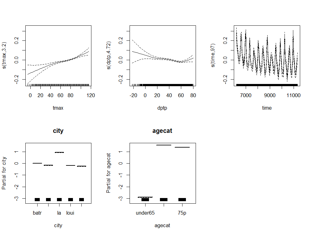
# name:core
# func
setwd("~/projects/spatiotemporal-regression-models/NMMAPS-example")
require(mgcv)
require(splines)

# load
analyte <- read.csv("analyte.csv")

# clean
analyte$yy <- substr(analyte$date,1,4)
numYears<-length(names(table(analyte$yy)))
analyte$date <- as.Date(analyte$date)
analyte$time <- as.numeric(analyte$date)
analyte$agecat <- factor(analyte$agecat,
                          levels = c("under65",
                              "65to74", "75p"),
                          ordered = TRUE
                          )

# do
fit <- gam(cvd ~ s(tmax) + s(dptp) +
           city + agecat +
           s(time, k= 7*numYears, fx=T) +
           offset(log(pop)),
           data = analyte, family = poisson
           )

# plot of response functions
png("images/nmmaps-eg-core.png", width = 1000, height = 750, res = 150)
par(mfrow=c(2,3))
plot(fit, all.terms = TRUE)
dev.off()

4.8.2 Core Model Plots

NMMAPS-example/images/nmmaps-eg-core.png

4.8.3 Model Selection

   
# The following codes are just a dump of stuff I've found useful in the past.
# This is all time-series methods.
# TODO replace the city-specific model with a pooled analysis with city specific trend.

# func
require(mgcv)
require(splines)
  
######################################################
# load  
dir("data")
city <- "Chicago"
data <- read.csv(sprintf("data/%s.csv", city), header=T)
str(data)
data$yy <- substr(data$date,1,4)
data$date <- as.Date(data$date)
######################################################
# check
par(mfrow=c(2,1), mar=c(4,4,3,1))
with(subset(data[,c(1,15:25)], agecat == '75p'),
  plot(date, tmax)
 )
with(subset(data[,c(1,4,15:25)], agecat == '75p'),
        plot(date, cvd, type ='l', col = 'grey')
        )
with(subset(data[,c(1,4,15:25)], agecat == '75p'),
        lines(lowess(date, cvd, f = 0.015))
        )
# I am worried about that outlier
data$date[which(data$cvd > 100)]
# [1] "1995-07-15" "1995-07-16"
 
######################################################
# do standard NMMAPS timeseries poisson GAM model
numYears<-length(names(table(data$yy)))
df <- subset(data, agecat == '75p')
df$time <- as.numeric(df$date)
fit <- gam(cvd ~ s(pm10tmean) + s(tmax) + s(dptp) + s(time, k= 7*numYears, fx=T), data = df, family = poisson)
# plot of response functions
par(mfrow=c(2,2))
plot(fit)
dev.off()
 
######################################################
# some diagnostics
summary(fit)
# note the R-sq.(adj) =   0.21
gam.check(fit)
# note the lack of a leverage plot.  for that we need glm
 
######################################################
# do same model as glm
fit2 <- glm(cvd ~ pm10tmean + ns(tmax, df = 8) + ns(dptp, df = 4) + ns(time, df = 7*numYears), data = df, family = poisson)
# plot responses
par(mfrow=c(2,2))
termplot(fit2, se =T)
dev.off()
 
# plot prediction
df$predictedCvd <- predict(fit2, df, 'response')
# baseline is given by the intercept
fit3 <- glm(cvd ~ 1, data = df, family = poisson)
df$baseline <-  predict(fit3, df, 'response')
with(subset(df, date>=as.Date('1995-01-01') & date <= as.Date('1995-07-31')),
 plot(date, cvd, type ='l', col = 'grey')
        )
with(subset(df, date>=as.Date('1995-01-01') & date <= as.Date('1995-07-31')),
        lines(date,predictedCvd)
        )
with(subset(df, date>=as.Date('1995-01-01') & date <= as.Date('1995-07-31')),
 lines(date,baseline)
        )
######################################################
# some diagnostics
# need to load a function to calculate poisson adjusted R squared
# original S code from
# The formula for pseudo-R^2 is taken from G. S. Maddalla,
# Limited-dependent and Qualitative Variables in Econometrics, Cambridge:Cambridge Univ. Press, 1983. page 40, equation 2.50.
RsquaredGlm <- function(o) {
 n <- length(o$residuals)
 ll <- logLik(o)[1]
 ll_0 <- logLik(update(o,~1))[1]
 R2 <- (1 - exp(((-2*ll) - (-2*ll_0))/n))/(1 - exp( - (-2*ll_0)/n))
 names(R2) <- 'pseudo.Rsquared'
 R2
 }
RsquaredGlm(fit2)
# 0.51
# the difference is presumably due to the arguments about how to account for unexplainable variance in the poisson distribution?
 
# significance of spline terms
drop1(fit2, test='Chisq')
# also note AIC. best model includes all of these terms
# BIC can be computed instead (but still labelled AIC) using
drop1(fit2, test='Chisq', k = log(nrow(data)))
 
# diagnostic plots
par(mfrow=c(2,2))
plot(fit2)
dev.off()
# note high leverage plus residuals points are labelled
# leverage doesn't seem to be too high though which is good
# NB the numbers refer to the row.names attribute which still refer to the original dataset, not this subset
df[row.names(df) %in% c(9354,9356),]$date
# as suspected [1] "1995-07-15" "1995-07-16"
 
######################################################
# so lets re run without these obs
df2 <- df[!row.names(df) %in% c(9354,9356),]
# to avoid duplicating code just re run fit2, replacing data=df with df2
# tmax still significant but not so extreme
# check diagnostic plots again
par(mfrow=c(2,2))
plot(fit2)
dev.off()
# looks like a well behaved model now.
 
# if we were still worried about any high leverage values we could identify these with
df3 <- na.omit(df2[,c('cvd','pm10tmean','tmax','dptp','time')])
df3$hatvalue <- hatvalues(fit2)
df3$res <- residuals(fit2, 'pearson')
with(df3, plot(hatvalue, res))
# this is the same as the fourth default glm diagnostic plot, which they label x-axis as leverage
summary(df3$hatvalue)
# gives us an idea of the distribution of hat values
# decide on a threshold and look at it
hatThreshold <- 0.1
with(subset(df3, hatvalue > hatThreshold), points(hatvalue, res, col = 'red', pch = 16))
abline(0,0)
segments(hatThreshold,-2,hatThreshold,15)
dev.off()
 
fit3 <- glm(cvd ~ pm10tmean + ns(tmax, df = 8) + ns(dptp, df = 4) + ns(time, df = 7*numYears), data = subset(df3, hatvalue < hatThreshold), family = poisson)
par(mfrow=c(2,2))
termplot(fit3, se = T)
# same same
plot(fit3)
# no better
 
# or we could go nuts with a whole number of ways of estimating influence
# check all influential observations
infl <- influence.measures(fit2)
# which observations 'are' influential
inflk <- which(apply(infl$is.inf, 1, any))
length(inflk)
 
 
######################################################
# now what about serial autocorrelation in the residuals?
 
par(mfrow = c(2,1))
with(df3, acf(res))
with(df3, pacf(res))
dev.off()
 
 
 
######################################################
# just check for overdispersion
fit <- gam(cvd ~ s(pm10tmean) + s(tmax) + s(dptp) + s(time, k= 7*numYears, fx=T), data = df, family = quasipoisson)
summary(fit)
# note the Scale est. = 1.1627
# alternatively check the glm
fit2 <- glm(cvd ~ pm10tmean + ns(tmax, df = 8) + ns(dptp, df = 4) + ns(time, df = 7*numYears), data = df, family = quasipoisson)
summary(fit2)
# (Dispersion parameter for quasipoisson family taken to be 1.222640)
# this is probably near enough to support a standard poisson model...
 
# if we have overdispersion we can use QAIC (A quasi- mode does not have a likelihood and so does not have an AIC,  by definition)
# we can use the poisson model and calculate the overdispersion
fit2 <- glm(cvd ~ pm10tmean + ns(tmax, df = 8) + ns(dptp, df = 4) + ns(time, df = 7*numYears), data = df, family = poisson)
1- pchisq(deviance(fit2), df.residual(fit2))
 
# QAIC, c is the variance inflation factor, the ratio of the residual deviance of the global (most complicated) model to the residual degrees of freedom
c=deviance(fit2)/df.residual(fit2)
QAIC.1=-2*logLik(fit2)/c + 2*(length(coef(fit2)) + 1)
QAIC.1
 
# Actually lets use QAICc which is more conservative about parameters,
QAICc.1=-2*logLik(fit2)/c + 2*(length(coef(fit2)) + 1) + 2*(length(coef(fit2)) + 1)*(length(coef(fit2)) + 1 + 1)/(nrow(na.omit(df[,c('cvd','pm10tmean','tmax','dptp','time')]))- (length(coef(fit2))+1)-1)
QAICc.1
 
 
######################################################
# the following is old work, some may be interesting
# such as the use of sinusoidal wave instead of smooth function of time
 
 
# # sine wave
# timevar <- as.data.frame(names(table(df$date)))
# index <- 1:length(names(table(df$date)))
# timevar$time2 <- index / (length(index) / (length(index)/365.25))
# names(timevar) <- c('date','timevar')
# timevar$date <- as.Date(timevar$date)
# df <- merge(df,timevar)
 
# fit <- gam(cvd ~ s(tmax) + s(dptp) + sin(timevar * 2 * pi) + cos(timevar * 2 * pi) + ns(time, df = numYears), data = df, family = poisson)
# summary(fit)
# par(mfrow=c(3,2))
# plot(fit, all.terms = T)
# dev.off()
 
# # now just explore the season fit
# fit <- gam(cvd ~ sin(timevar * 2 * pi) + cos(timevar * 2 * pi) + ns(time, df = numYears), data = df, family = poisson)
# yhat <- predict(fit)
# head(yhat)
 
# with(df, plot(date,cvd,type = 'l',col='grey', ylim = c(15,55)))
# lines(df[,'date'],exp(yhat),col='red')
 
 
# # drop1(fit, test= 'Chisq')
 
# # drop1 only works in glm?
# # fit with weather variables, use degrees of freedom estimated by gam
# fit <- glm(cvd ~ ns(tmax,8) + ns(dptp,2) + sin(timevar * 2 * pi) + cos(timevar * 2 * pi) + ns(time, df = numYears), data = df, family = poisson)
# drop1(fit, test= 'Chisq')
# # use plot.glm for diagnostics
# par(mfrow=c(2,2))
# plot(fit)
# par(mfrow=c(3,2))
# termplot(fit, se=T)
# dev.off()
 
# # cyclic spline, overlay on prior sinusoidal
# with(df, plot(date,cvd,type = 'l',col='grey', ylim = c(0,55)))
# lines(df[,'date'],exp(yhat),col='red')
 
# df$daynum <- as.numeric(format(df$date, "%j"))
# df[360:370,c('date','daynum')]
# fit <- gam(cvd ~ s(daynum, k=3, fx=T, bs = 'cp') +  s(time, k = numYears, fx = T), data = df, family = poisson)
# yhat2 <- predict(fit)
# head(yhat2)
 
# lines(df[,'date'],exp(yhat2),col='blue')
 
 
# par(mfrow=c(1,2))
# plot(fit)
 
 
# # fit weather with season
# fit <- gam(cvd ~ s(tmax) + s(dptp) +
  # s(daynum, k=3, fx=T, bs = 'cp') +  s(time, k = numYears, fx = T), data = df, family = poisson)
# par(mfrow=c(2,2))
# plot(fit)
 
# summary(fit)

5 Spatial lag and timeseries

I will use the same NMMAPSlite to show how I'd approach a simple "Spatio-Temporal" model.

TODO The following is a stub of an idea. For further development

5.1 Data

5.1.1 Zones

Spatial Neighbours Code

################################################################
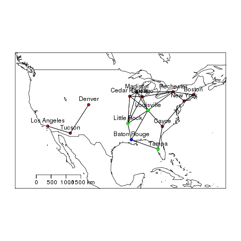
# name:spatwat
# func
setwd("~/projects/spatiotemporal-regression-models/NMMAPS-example")
require(gisviz)

# load
dir()
shp <- readOGR("cities.shp", "cities")

# clean
head(shp@data)

# do
## I will use nearest neighbour within a distance threshold, but
## usually polygon datasets would use poly2nb
nb <- dnearneigh(shp, d1 = 1, d2 = 1000)                      
head(nb)
shp[[1]][1]
shp[[1]][nb[[1]]]
# map
nudge <- 10
png("images/nmmaps-eg-neighbourhood.png")
plotMyMap(
    shp@coords, xl = c(min(shp@coords[,1])-nudge, max(shp@coords[,1])+nudge),
    yl = c(min(shp@coords[,2])-nudge, max(shp@coords[,2])+nudge)
    )
plot(nb, shp@coords, add=TRUE)
text(shp@data$long, shp@data$lat, shp@data$address, pos=3)
points(shp@coords[nb[[1]],], col = 'green', pch = 16)
points(shp@data[1,c("long","lat")],col = 'blue', pch = 16)
dev.off()

Spatial Neighbours Output

5.1.2 Outcome

#### Now do the Neighbourhood autoregressive lagged variable  ####
# func
setwd("~/projects/spatiotemporal-regression-models/NMMAPS-example")
require(gisviz)
require(plyr)

# load
analyte <- read.csv("analyte.csv")
shp <- readOGR("cities.shp", "cities")

# clean
analyte$yy <- substr(analyte$date,1,4)
numYears<-length(names(table(analyte$yy)))
analyte$date <- as.Date(analyte$date)
analyte$time <- as.numeric(analyte$date)
analyte$agecat <- factor(analyte$agecat,
                          levels = c("under65",
                              "65to74", "75p"),
                          ordered = TRUE
                          )
 
names(analyte)
analyte[1,]
table(analyte$city)
# do
study <- analyte[, c("city","date", "agecat", "cvd", "pop")]
subset(study, city == "tucs" & date == as.Date("1991-01-01"))

nb <- dnearneigh(shp, d1 = 1, d2 = 1000)                      
head(nb)
head(shp@data)
adj <- adjacency_df(NB = nb, shp = shp, zone_id = 'city')
subset(adj, V1 == "tucs")

neighbours <- merge(study, adj, by.x = "city", by.y = "V1")
subset(neighbours, city == "tucs" & date == as.Date("1991-01-01"))

xvars <- c("V2", "date","agecat")
yvars <- c("city", "date", "agecat")
neighbours <- merge(neighbours[,c(xvars, "city")],
                    analyte[,c(yvars, "cvd", "pop")],
                    by.x = xvars,
                    by.y = yvars)
names(neighbours)
subset(neighbours, city == "tucs" & date == as.Date("1991-01-01"))

neighbours$asr  <- (neighbours$cvd / neighbours$pop) * 1000


neighbours2  <- ddply(neighbours, c("city", "date", "agecat"), summarise,
                     NeighboursYij  = mean(asr)
                     )
subset(neighbours2, city == "tucs" & date == as.Date("1991-01-01"))
table(neighbours2$city)
head(analyte)

analyte  <- merge(analyte, neighbours2, by = c("city", "agecat", "date"))
analyte <- arrange(analyte, city, date, agecat)
head(analyte)

5.2 Analysis

5.2.1 Model with Spatial Lag

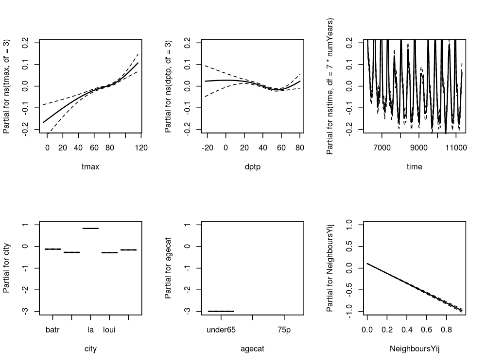
# func
require(splines)

# load
# assumes the prior code chunks have been run

# do
fit <- glm(cvd ~ ns(tmax, df = 3) + ns(dptp, df = 3) +
           NeighboursYij + 
           city + agecat +
           ns(time, df = 7*numYears) +
           offset(log(pop)),
           data = analyte, family = poisson
           )

# plot of response functions
png("images/nmmaps-eg-sp-lag.png", width = 1000, height = 750, res = 150)
par(mfrow=c(2,3))
termplot(fit, terms = attr(terms(fit),'term.labels') [c(1:2,6)], se = TRUE, ylim =c(-.2,.2), col.term = 'black', col.se = 'black')
termplot(fit, terms = attr(terms(fit),'term.labels') [c(4,5)], se = TRUE, ylim =c(-3,3), col.term = 'black', col.se = 'black')
termplot(fit, terms = attr(terms(fit),'term.labels') [3], se = TRUE, ylim =c(-1,1), col.term = 'black', col.se = 'black')
dev.off()

5.2.2 Spatial Lag Model Plots

NMMAPS-example/images/nmmaps-eg-sp-lag.png